code

share


In this Section we introduce the general framework of nonlinear regression, along with many examples ranging from toy datasets to classic examples from differential equations. These examples are all low dimensional, allowing us to visually examine patterns in the data and propose appropriate nonlinearities, which we can (as we will see) very quickly inject into our linear supervised paradigm to produce nonlinear regression fits. By walking through these examples we flush out a number important concepts in concrete terms, coding principles, and jargon-terms in a relatively simple environment that will be omnipresent in our discussion of nonlinear learning going forward.
In Chapter 8 we discussed linear regression, where we began with a very particular ideal desire to relate the input/output of a given dataset linearly as
\begin{equation} w_0 + x_{1,p}w_1 + \cdots + x_{N,p}w_N \approx y_p \end{equation}where the input $\mathbf{x}_p = \begin{bmatrix} x_{1,p}\\ \vdots \\ x_{N,p} \end{bmatrix}$ and output $y_p$ is the $p^{th}$ datapoint from a set of $P$ such points and $w_0$ is the bias and $w_1,\,w_2,\,...,\,w_N$ the slope parameters of our linear model. This was our ideal scenario, that is, when these weights were tuned properly they all lie close to a particular hyperplane defined by the ideal weights.
The linear modeling assumption enters on the left side of each $\approx$ sign, our model which takes in a datapoint $\mathbf{x}_p$ and outputs a value we hope matches $y_p$ closely. We can write our linear predictor more generically as
\begin{equation} \text{model}\left(\mathbf{x},\mathbf{w}\right) = w_0 + x_{1}w_1 + \cdots + x_{N}w_N \end{equation}or more compactly in various ways e.g., as $\text{model}\left(\mathbf{x},\mathbf{w}\right) = \mathring{\mathbf{x}}^T \mathbf{w}^{\,}$ where we use our 'compact' notation denoting
\begin{equation} \mathbf{w}=\begin{bmatrix} w_{0}\\ w_{1}\\ w_{2}\\ \vdots\\ w_{N} \end{bmatrix} \,\,\,\,\,\,\,\,\,\,\,\,\,\,\,\,\,\,\,\,\,\,\,\,\,\,\,\,\,\,\,\, \mathring{\mathbf{x}}=\begin{bmatrix} 1 \\ x_{1}\\ w_{2}\\ \vdots\\ w_{N} \end{bmatrix},\,\,\,\, \end{equation}In Section 8.1.3 we implemented this linear model compactly in Python - allowing us to evaluate an entire dataset at once as shown below.
# compute linear combination of input point
def model(x,w):
    # tack a 1 onto the top of each input point all at once
    o = np.ones((1,np.shape(x)[1]))
    x = np.vstack((o,x))

    # compute linear combination and return
    a = np.dot(x.T,w)
    return a.T
In our model notation we can express equation (1) as
Moreover as we saw in our discussion of Least Squares linear regression in Section 8.1 the ideal scenario expressed above naturally leads to a Least Squares cost function
\begin{equation} g\left(\mathbf{w}\right) = \frac{1}{P}\sum_{p=1}^{P}\left(\text{model}\left(\mathbf{x}_p,\mathbf{w}\right) - y_p\right)^2 \end{equation}whose minimum provides us with the weights that service our ideal as best as possible.
When first introducing this notation in Section 8.1.3 we discussed how separating out the model allowed us to both think about and implement linear regression cost functions in a more modular manner. However it allows us directly move from linear to general nonlinear regression - in both its principles and implementation - with few obstacles. How? We simply swap out the linear model used in the construction of our regression - e.g., in equations (4) and (5) above - with a nonlinear one. Indeed beginning with the principle we started with, beginning with the ideal scenario in equation (4) where we suppose we have perfect weights and ending with the Last Squares cost function in equation (5) for recovering them, we can see that there was nothing particular to this argument demanded that our model be a linear one. This was an assumption we made - we chose a linear model to perform regression with.
So instead of using a linear model we could instead use a nonlinear one, involving a single nonlinear function $f$ that can be parameterized or unparameterized (e.g., tanh, a sine wave, etc.,) as
\begin{equation} \text{model}\left(\mathbf{x},\mathbf{w}\right) = w_0^{\,} + f\left(\mathbf{x}_p\right){w}_{1}^{\,}. \end{equation}In the jargon of machine learning / deep learning the nonlinear function $f$ is often called a nonlinear feature transformation, since we it transforms our original input features $\mathbf{x}$.
In the jargon of machine learning / deep learning a nonlinear function $f$ used in any learning
modelis called a nonlinear feature transformation, since we it transforms our original input features $\mathbf{x}$.
Again we could consider the ideal case - where we have knowledge of the best possible weights so that
\begin{equation} \text{model}\left(\mathbf{x}_p,\mathbf{w}\right) \approx y_p \end{equation}and to recover our ideal weights we would follow the same logic as previously: square the difference between both sides of the above and sum over all the points, giving the Least Squares cost function $ g\left(\mathbf{w}\right) = \frac{1}{P}\sum_{p=1}^{P}\left(\text{model}\left(\mathbf{x}_p,\mathbf{w}\right) - y_p\right)^2 $ that - when minimized properly - still minimizes a squared error of our (now nonlinear) model and provides us with our desired weights.
Indeed in general we could create a nonlinear model that is the weighted sum of $B$ nonlinear functions of our input as
\begin{equation} \text{model}\left(\mathbf{x},\mathbf{w}\right) = w_0 + f_1\left(\mathbf{x}_p\right){w}_{1} + f_2\left(\mathbf{x}_p\right){w}_{2} + \cdots + f_B\left(\mathbf{x}_p\right)w_B \end{equation}where $f_1,\,f_2,\,...\,f_B$ are nonlinear parameterized or unparameterized functions - or feature transformations - and $w_0$ through $w_B$ (along with any additional weights internal to the nonlinear functions) are represented in the weight set $\mathbf{w}$ and must be tuned properly. Nonetheless the steps we take to formally employ such a model, its ideal weight values, the derivation of a Least Squares cost function, etc., are entirely similar to what we have now seen in the simpler instance of nonlinear regression (which itself does not differ from the steps taken in modeling the linear case).
In extending linear to nonlinear regression we can use either parameterized or unparameterized nonlinear functions
In this Subsection we walk through a number of simple examples of nonlinear regression where we can determine - by eye - a proper nonlinear model to use. We then show how to implement and optimize each model by minimizing the corresponding Least Squares cost function. These examples also allow us to introduce a number of important principles, formulations, and jargon-terms - that we will see considerably more of when discussing neural networks, tree-based learners, and kernels - in a comparatively simple context.
In terms of implementation, every example that follows employs the same least_squares function we first detailed in Section 8.1, and shown below (we can also use other cost functions for regression as well like e.g., the Least Absolute Deviation cost described in Section 8.3).
# an implementation of the least squares cost function for linear regression
def least_squares(w):
    cost = np.sum((model(x,w) - y)**2)
    return cost/float(len(y))
For each example that follows our model implementation will also look very similar to its original version first shown in Section 8.1, with one very important new line. We now compute desired feature transformations of the input $\mathbf{x}$ - which will also take in parameters depending on the particular feature transformations employed - via the Python function called feature_transforms. The implementation of model below is written generically for the case where our desired feature transformations have internal parameters (hence why feature_transforms takes in the set of weights assigned to w[0], with the weights in the final linear combinatin of the model stored in w[1]). If - for example - the feature transformations being used do not have internal parameters the call to feature_transforms in line 4 below would instead look like
f = feature_transforms(x)
and the linear combination of transformed features in line 11 instead
a = np.dot(f.T,w)# an implementation of our model employing a nonlinear feature transformation
def model(x,w):
# feature transformation
f = feature_transforms(x,w[0])
# tack a 1 onto the top of each input point all at once
o = np.ones((1,np.shape(f)[1]))
f = np.vstack((o,f))
# compute linear combination and return
a = np.dot(f.T,w[1])
return a.T
Since these blocks of code will be generally the same across our examples we will not repeat them so that we can focus our attention in each case on how to implement particular feature transformations as the Python function feature_transforms. We will employ these functions - along with the normalization modules and gradient descent optimizer we have implemented in previous Chapters - via a backend file basic_runner.py.
As a first and simple example we can write the feature_transforms function for the simple case of linear regression and see how it can be directly plugged into our model, tuned, etc., Below we load in a dataset that clearly looks like a linear model would fit well if its parameters were properly tuned.

Here we would propose to use the standard sort of linear model we saw in previous Chapters
\begin{equation} \text{model}\left(x,\mathbf{w}_{\!}\right) = w_0 + xw_1. \end{equation}Here - although we did not explicitly call it such - we are employing the simple linear feature transformation
\begin{equation} f\left(x\right) = x \end{equation}and in this notation our model is then equivalently
This is a rather trivial feature transformation to implement in Python - as we do below. Notice here how the linear feature transformation is unparameterized.
# the trivial linear feature transformation
def feature_transforms(x):
    return x
Below we perform a run of gradient descent on this dataset - first performing standard normalization on the input as detailed in Section 8.4. Performing standard normalization (subtracing the mean and dividing off the standard deviation of the input) we can actually think of the normalization as being a part of the feature transformation itself, and write it formally as
\begin{equation} f\left(x \right) = \frac{x - \mu}{\sigma} \end{equation}where $\mu$ and $\sigma$ are the mean and standard deviation of the dataset's input. There is no need however to adjust the feature_transforms implementation to reflect this, since we can construct this version of our feature transformation by composing it with a function normalizer function that performs the standard normalization (as detailed in e.g., Section 8.4) as feature_transforms(normalizer(x)).
We can then plot the line correspnoding to those weights providing the lowest cost function value during the run, as we do below. The fit does indeed match the behavior of the dataset well.

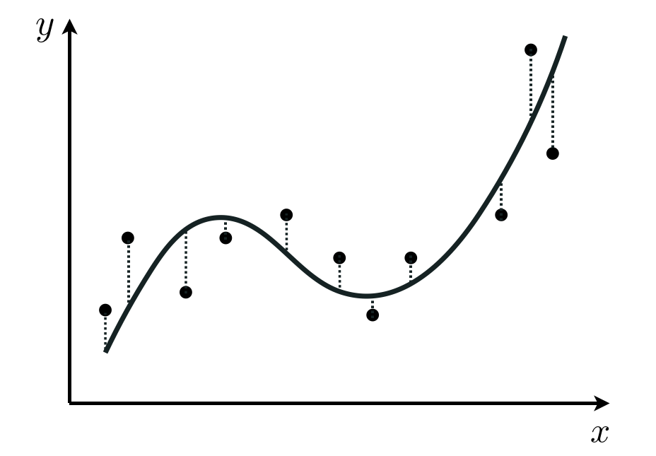
Lets look at the following wavy looking regression dataset, postulate an appropriate nonlinear model, implement it and fit it to the data by minimizing the corresponding Least Squares cost.

This dataset looks sinusoidal, so we can defensibly propose a model consisting of completely parameterized sine function or feature transformation
We can then take as our model a linear combination of this nonlinear feature transformation as
\begin{equation} \text{model}\left(x,\mathbf{w}_{\!}\right) = w_2 + f\left(x,\mathbf{w}\right)w_{3\,}. \end{equation}Note here we are using the notation $\mathbf{w}$ rather loosely to represent whatever weights are present in the respective formula - for example in the feature transformation $\mathbf{w}$ consists of $w_0$ and $w_1$, whereas with the model it contains these weights as well as $w_2$ and $w_3$.
This seems like it could fit the data well if its parameters were all tuned properly via e.g., minimizing the associated Least Squares cost. However first we need to implement our feature transformation in Python, which we will do below.
# our nonlinearity, known as a feature transformation
def feature_transforms(x,w):
    # tack a 1 onto the top of each input point all at once
    o = np.ones((1,np.shape(x)[1]))
    x = np.vstack((o,x))

    # calculate feature transform
    f = np.sin(np.dot(x.T,w)).T
    return f
Below we make a run of gradient descent on the original and standard normalized versions of the input, and compare their cost function histories afterwards. Input normalization - discussed in the context of linear regression in Sections 8.4 and 11.3 - is equally important in the context of nonlinear regression (we will have much more to say on this topic in future Sections) in terms of tempering the contours of any regression cost function making it considerably easier for gradient descent to minimize.
Now we compare the cost function histories of each run in the cost function plot below. This sort of result is very typical of nonlinear regression and while we will not normalize the input of every toy example discussed in this and the next Sections for reasons of clarity, it serves as an important reminder that in practice one should never forget to normalize input when tuning a nonlinear supervised learner via gradient descent. The run on the original data is actually somewhat deceiving here - it converges but not to the global minimum achieved using the normalized input.

We can then plot the resulting fit to the data provided by the run on the normalized input - and achieve quite a good fit.

Note as with the previous example that since we have used standard normalization to scale our input, we can write our feature transformation as
\begin{equation} f\left(x,\mathbf{w}\right) = \text{sin}\left(w_0 + \frac{x - \mu}{\sigma}w_1\right) \end{equation}where $\mu$ and $\sigma$ are the mean and standard deviation of our input data respectively. Once again we need not adjust our actual implementation feature_transforms, since we accomplish this formula in Python by composing the function with the standard normalizer function as feature_transforms(normalizer(x)).
With our weights fully tuned to our ideal parameters $\mathbf{w}^{\star}$ notice that since model is defined linearly in terms of its feature transformation we can represent our transformed input $x_p \longleftarrow f\left(x_p,\mathbf{w}^{\star}\right)$ and the correspnoding model fit $
\text{model}\left(x,\mathbf{w}^{\star}\right)$ in what is called the transformed feature space. This is simply the space whose input is the feature transformed input $\left(x,\mathbf{w}^{\star}\right)$ and whose output remains as $y$. In this space our nonlinear fit is a linear one. In other words, with our model completely tuned if plot the points $\left(f\left(x_1,\mathbf{w}^{\star}\right),y_1\right),\,\left(f\left(x_2,\mathbf{w}^{\star}\right),y_2\right)...,\left(f\left(x_P,\mathbf{w}^{\star}\right),y_P\right)$ - as we do below in the right panel - our model fits the transformed data linearly.
This finding is true in general with nonlinear regression problems.
A properly designed feature (or set of features) provides a good nonlinear fit in the original feature space and, simultaneously, a good linear fit in the transformed feature space.

Next we examine a population growth dataset - which shows the population of Yeast cells growing in a constrained chamber (you can find the source of this dataset here). This is a common shape found with population growth data, where the creature under study starts off with only a few members and is only limited in growth by how fast it can reproduce and the resources available in its environment. In the beginning such a population grows exponentially. This growth halts rapidly when the population reaches the maximum carrying capacity of its environment.

If we take a moment and visually examine this dataset, it appears that some sort of logistic sigmoid / hyperbolic tangent nonlinearity would fit it quite well. So using a parameterized tanh feature transformation
\begin{equation} f\left(x,\mathbf{w}\right) = \text{tanh}\left(w_0 + xw_1\right). \end{equation}we can then take as our model a linear combination of this nonlinear feature transformation as
Note here we are using the notation $\mathbf{w}$ rather loosely to represent whatever weights are present in the respective formula - for example in the feature transformation $\mathbf{w}$ consists of $w_0$ and $w_1$, whereas with the model it contains these weights as well as $w_2$ and $w_3$.
Below we show an implementation of this feature transformation and associated model.
# our nonlinearity, known as a feature transformation
def feature_transforms(x,w):
    # tack a 1 onto the top of each input point all at once
    o = np.ones((1,np.shape(x)[1]))
    x = np.vstack((o,x))

    # calculate feature transform
    f = np.tanh(np.dot(x.T,w)).T
    return f
Using the same functionality employed in the previous example, we normalize the input of this dataset (using standard normalization) since this virtually always helps speed up gradient descent significantly. Note this means that our feature transformation can be written as
\begin{equation} f\left(x_p,\mathbf{w}\right) = \text{tanh}\left(w_0 + \frac{x_p - \mu}{\sigma}w_1\right) \end{equation}where $\mu$ and $\sigma$ are the mean and standard deviation of our input data respectively. We do not need to alter our feature transformation code above make this change, since it can be accomplished by feeding in the normalized input for training and the corresponding normalization function while evaluating test points.
Below we then form the corresponding Least Squares cost, and minimize it using gradient descent.
To check the convergence of our run of gradient descent we show the corresponding cost function history plot below.

With our minimization complete we can then fit our model function in both the original space (where it provides a good nonlinear fit) as well as in the transformed feature space where it simultaneously provides a good linear fit to the transformed data (as discussed in the previous example).

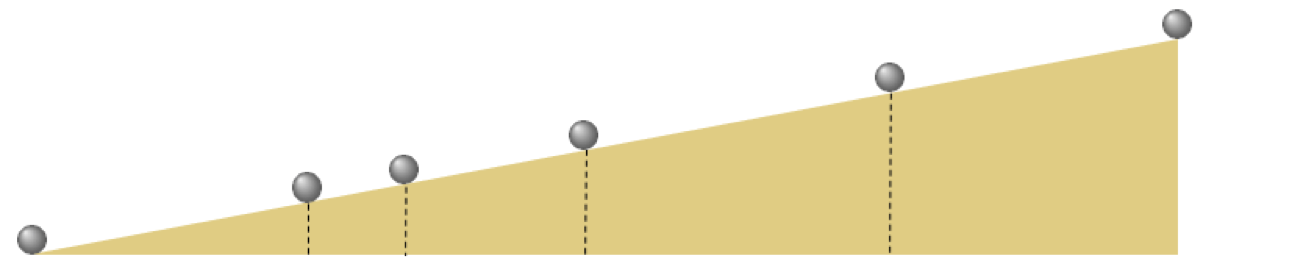
In 1638 Galileo Galilei, infamous for his expulsion from the Catholic church for daring to claim that the earth orbited the sun and not the converse (as was the prevailing belief at the time) published his final book: Discourses and Mathematical Demonstrations Relating to Two New Sciences. In this book, written as a discourse among three men in the tradition of Aristotle, he described his experimental and philosophical evidence for the notion of uniformly accelerated physical motion. Specifically, Galileo (and others) had intuition that the acceleration of an object due to (the force we now know as) gravity is uniform in time, or in other words that the distance an object falls is directly proportional (i.e., linearly related) to the amount of time it has been traveling, squared. This relationship was empirically solidified using the following ingeniously simple experiment performed by Galileo.
Repeatedly rolling a metal ball down a grooved $\frac{1}{2}$ meter long piece of wood set at an incline as shown in the Figure below, Galileo timed how long the ball took to get $\frac{1}{4}$,$\frac{1}{2}$, $\frac{2}{3}$, $\frac{3}{4}$, and all the way down the wood ramp.
Why didn't Galileo simply drop the ball from some height and time how long it took to reach certain distances to the ground? Because no reliable way to measure time yet existed (he had to use a water clock for these experiments)! Galileo was the one who set humanity on the route towards its first reliable time-piece in his studies of the pendulum
Data from a (modern reenactment) of these experiments (averaged over 30 trials), results in the 6 data points shown below. Here the input axis is the number seconds while the output is the portion of the ramp traveled by the ball during the experiments.

The data here certainly displays a nonlinear relationship and by viewing it - and using his physical intuition Galileo - intuited a quadratic relationship. Or in our jargon that for some $w_0$, $w_1$, and $w_2$ the modeling function
\begin{equation} \text{model}(x,\mathbf{w}) = w_0 + xw_1 + x^2w_2 \end{equation}provides the correct sort of nonlinearity to explain this data (albeit when the parameters are tuned correctly).
Notice here how we have two unparameterized feature transformations: the identity $f_1(x) = x$ and the quadratic term $f_2(x) = x^2$, and so we may write the above equivalently as
\begin{equation} \text{model}(x,\mathbf{w}) = w_0 + f_1(x)\,w_1 + f_2(x)\,w_2 \end{equation}which clearly shows how we are seeking out a proper linear relationship in the transformed feature space (which in this case is two-dimensional). Note here - unlike the previous examples - neither of these feature transformations are fixed in that they take in no internal weights.
Below implement both feature transformations in a single Python function, the model function.
def feature_transforms(x):
    # calculate feature transform
    f = np.array([(x.flatten()**d) for d in range(1,3)])
    return f
As in the previous examples we perform standard normalization on the input of this dataset to speed up gradient descent. This means that we can think of each of our feature transformations as involving this form of normalization as $f_1(x) = \frac{x - \mu}{\sigma}$ and the quadratic term $f_2(x) = \left(\frac{x - \mu}{\sigma}\right)^2$ where $\mu$ and $\sigma$ are the mean and standard deviation of the input data, which we accomplish by feeding normalized input into each.
Now we can plot our original data and nonlinear fit in the original space (left panel below), as well as transformed data and simultaneous linear fit in the transformed feature space (right panel below). Notice that since we have two features in this instance our linear fit is in a space one dimension higher than the original input space defined by $x$. In other words, the transformed feature space here has two inputs: one defined by each of the two features $f_1$ and $f_2$.

This is true more generally speaking: the more feature transforms we use the higher the up we go in terms of the dimensions of our transformed feature space / linear fit! In general if our original input has dimension $N$ - and is written as $\mathbf{x}$ - and we use a model function that employs $B$ nonlinear feature transformations as
then our original space has $N$ dimensional input, while our transformed feature space is $B$ dimensional. Note here that the set of all weights $\omega$ contains not only the weights $w_1,\,w_2,...,w_B$ from the linear combination, but also any features's internal parameters as well.