code

share


In this Section we introduce the general framework of nonlinear unsupervised learning. Since there are such a wide variety of unsupervised learning models (see Chapter 11), and we want to keep things as elementary as we can in this Section, here we will focus our attention exclusively on how to extend perhaps the most important linear unsupervised learner to the nonlinear setting: the PCA autoencoder (detailed in Section 11.2). In future Chapters we will look at particular examples of how to extend other unsupervised methods such as K-Means.
In Section 11.2 we discussed the PCA autoencoder, the fundamental cost function for PCA that leads to the classic orthogonal PCA solution (described in Section 11.2.3). The autoencoder cost function
\begin{equation} g\left(\mathbf{C}\right) = \frac{1}{P}\sum_{p = 1}^P \left \Vert \mathbf{C}_{\,}^{\,}\mathbf{C}_{\,}^T\mathbf{x}_p - \mathbf{x}_p \right\Vert_2^2 \end{equation}is parameterized by the $N\times K$ matrix $\mathbf{C}$ that will act as our recovered basis upon minimization.
In preparation for the nonlinear extension of this scheme - which we will use to determine proper nonlinear manifolds for an input dataset - we will explicitly break up $\mathbf{C}\mathbf{C}^T\mathbf{x}_p$ into an explicit encoding and decoding step. We have our encoder function $f_{\text{e}}$
and decoder function $f_{\text{d}}$
We can then write our two linear operations on the input with this function notation as
\begin{equation} f_{\text{d}}\left(\,f_{\text{e}}\left(\mathbf{x}_p\right)\right) = \mathbf{C}_{\,}^{\,}\mathbf{C}_{\,}^T\mathbf{x}_p \end{equation}where note here that notationally speaking we have left off dependency on internal parameters with the aim of keeping our formula simple and more understandable, so e.g., here to make each function visibly dependent on the parameters $\mathbf{C}$ we would write $f_{\text{d}}\left(\mathbf{v},\mathbf{C}\right)$ and $f_{\text{e}}\left(\mathbf{x},\mathbf{C}\right)$.
We can then write the autoencoder cost function with this more general function notation as
This sort of mathematical notation carries over almost directly to Python, as we show below. Here we process the entire dataset $\mathbf{X}$ in one operation (which is more effecient in Python than explicitly looping over the points). Notice in both implementations - as opposed to the notation used above - we input C as well as the data.
# a linear encoder function
def encoder(X,C):
    return np.dot(C.T,X)

# a linear decoder function
def decoder(V,C):
    return np.dot(C,V)
In order to wrap up these two functions we can then use our typical model function, as shown below. Running this on a single $\mathbf{x}$ produces the entire computation $f_{\text{d}}\left(\,f_{\text{e}}\left(\mathbf{x}_p\right)\right)$.
# a model function wrapping up our linear encoding/decoding schemes
def model(X,C):
    # encode the input
    V = encoder(X,C)

    # decode the encoding
    a = decoder(V,C)
    return a
To tune these parameters properly we can then minimize the autoencoder function below using e.g., gradient descent.
# an implementation of the least squares cost function for linear regression
def autoencoder(C):
    cost = np.sum((model(X,C) - X)**2)
    return cost/float(X.shape[1])
Here we re-enact an experiment showing how to use the standard linear autoencoder first shown in Section 11.4, employing the organizatinoal style detailed above, to find the best one dimensional subspace for the two dimensional dataset shown below.

In visually examining this dataset it does indeed look like it could be reasonably represented using a linear manifold or subspace (which in this case is clearly a line). Because of this we can use our linear encoder and decoder functions defined above.
Using gradient descent we then minimize the autoencoder cost, finding the best one dimensional subspace for this two-dimensional dataset.
Shown below in the top row is (left panel) the original data and the principal component recovered (shown as a red arrow), the encoded version (middle panel) and decoded version (right panel) of the input data along with the subspace spanned by the recovered basis vector. In the bottom row we show the manifold recovered - as a black line with red outline for visualization purposes - and illustrate how points in the space are attracted to the recovered manifold as a vector field with arrows colored according to their distance to the linear subspace.


Now just as we discussed in the previous Sections, where we described how to extend linear regression and classification to the general nonlinear case, here the fact the encoder and decoder above are linear does not reflect a limitation of the autoencoder framework but simply modeling choice of ours. We (originally) aimed to uncover the best linear subspace for an input dataset because this is the simplest model to work with, and allows us to flush out important technical details. However nothing about the autoencoder framework itself limits us to using linear encoding/decoding functions, and thus prevents us from extending the idea in order to uncover the best nonlinear manifold for a given set of input data.
In general we want an encoder/decoder pair so that
\begin{equation} f_{\text{d}}\left(\,f_{\text{e}}\left(\mathbf{x}_p\right)\right) \approx \mathbf{x}_p \end{equation}In other words - we aim for our encoder/decoder pair to learn an identity function for our given input.
To make this extension we can introduce any two parameterized nonlinear functions: one for encoding $\,\,f_{\text{e}}\left(\mathbf{x}\right)$ and one for decoding $ f_{\text{d}}\left(\mathbf{v}\right)$ (again leaving off explicit dependency on internal parameters with both functions for notational simplicity). Each of these can be a nonlinear feature transformation or linear combination of $B$ such transformations, e.g., in general our encoder can take the form
where $f_1,\,f_2,\,...\,f_B$ are nonlinear parameterized or unparameterized feature transformations and $w_0$ through $w_B$ - as well as any weights internal to the nonlinear functions - must be tuned properly. We can likewise think of the general decoder function $f_{\text{d}}\left(\mathbf{v}\right)$ this way as well.
If we swap out our linear encoding/decoding schemes for these more general functions we have a general autoencoder function
\begin{equation} g\left(\mathbf{w}\right) = \frac{1}{P}\sum_{p = 1}^P \left \Vert \,f_{\text{d}}\left(\,f_{\text{e}}\left(\mathbf{x}_p\right)\right) - \mathbf{x}_p \right\Vert_2^2 \end{equation}where we have denoted by $\mathbf{w}$ the entire set of parameters of both the encoder $f_{\text{e}}$ and decoder $f_\text{d}$. In the linear case we have $\mathbf{w} = \mathbf{C}$. Note we could also use a linear combination of nonlinear feature transformations for both encoder and decoder as well.
To implement the nonlinear autoencoder in Python we can virtually re-use most of the code framework we employed in the linear case - including our model and autoencoder functions. We only need to slightly modify the model function to take in a generally larger set of parameters - since each of our encoding/decoding functions can in general have unique sets of parameters. To keep things as general as possible we will rewrite the model function as shown below. Note here we input a single list w which contains two arrays: its first array w[0] contains the parameters of our encoder while the second array w[1] contains parameters of the decoder. The encoder and decoder's sets of parameters can be identical (as with the linear case discussed in the previous Subsection), partially overlap, or be completely disjoint.
# a general model wrapping up our encoder/decoder
def model(X,w):
    # encode the input
    v = encoder(X,w[0])

    # decode the encoding
    a = decoder(v,w[1])
    return a
Then since each of our encoder and decoder function can in general be a linear combination of feature transformations, each can be written in general precisely as we implemented a single such combination of features for e.g., regression or classification in the previous two Sections. For example, in general the encoder can be implemented as follows (and likewise for the general decoder).
# an implementation of our model employing a nonlinear feature transformation
def encoder(x,w):
    # feature transformation
    f = feature_transforms(x,w[0])

    # tack a 1 onto the top of each input point all at once
    o = np.ones((1,np.shape(f)[1]))
    f = np.vstack((o,f))

    # compute linear combination and return
    a = np.dot(f.T,w[1])
    return a.T
In short, to use the nonlinear autoencoder we need only define encoder and decoder functions, since the above autoencoder cost function implementation is always the same regardless of the dataset/nonlinearities used and model functions will always be more or less the same.
# an implementation of the least squares cost function for linear regression
def autoencoder(w):
    cost = np.sum((model(X,w) - X)**2)
    return cost/float(X.shape[1])
In this example we use a simulated dataset of $P=20$ two-dimensional data points to learn a circular manifold via our nonlinear autoencoder scheme. The Python cell below plots the data - which as you can see - has an almost circular shape but not all of the data points fall precisely on a circle (due to noise).

A general circle in 2-d, as shown in the left panel of Figure 1, can be characterized using its center point $\mathbf{w}$ and radius $r$. Subtracting off $\mathbf{w}$ from any point $\mathbf{x}_p$ on the circle then centers the data at origin, as shown in the right panel of Figure 1.
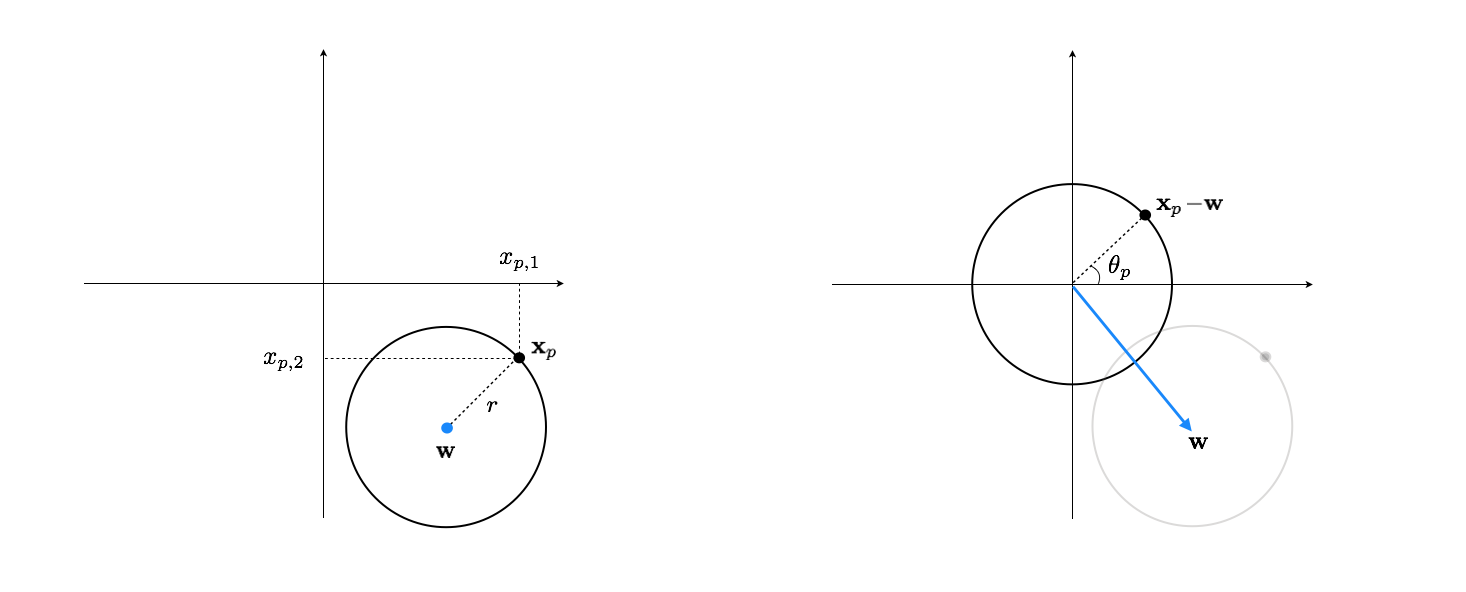
Once centered, any two-dimensional data point $\mathbf{x}_p-\mathbf{w}$ on the circle can be encoded as the (scalar) angle $\theta_p$ between the line segment connecting it to the origin and the horizontal axis. Mathematically speaking we have
\begin{equation} \theta_p=\text{arctan}\left(\frac{x_ {p,2}-w_2}{x_{p,1}-w_1}\right) \end{equation}This is our nonlinear encoder which we implement below along with our custom arctan function.
def my_arctan(x1,x2):
    v = x2/x1
    if x1 > 0:
        return np.arctan(v)
    elif x1 < 0 and x2 >= 0:
        return np.arctan(v) + np.pi
    elif x1 < 0 and x2 < 0:
        return np.arctan(v) - np.pi
    elif x1==0 and x2 > 0:
        return np.pi*0.5
    elif x1==0 and x2 < 0:
        return -np.pi*0.5

def encoder(x,w):
    a = x - w
    b = []
    for i in range(a.shape[1]):
        b.append(my_arctan(a[0][i],a[1][i]))
    b = np.array(b)[np.newaxis,:]
    return b
To design the decoder, beginning with $\theta_p$, we can reconstruct $\mathbf{x}_p$ as
\begin{equation} \mathbf{x}_p=\left[\begin{array}{c} r_1\,\text{cos}(\theta_p)+w_1\\ r_2\,\text{sin}(\theta_p)+w_2 \end{array}\right] \end{equation}The decoder function below implements this nonlinear decoding process.
def decoder(v,w):
    a = w[:,0][:,np.newaxis]*np.vstack((np.cos(v),np.sin(v))) + w[:,1][:,np.newaxis]
    return a
Using gradient descent we can now minimize the autoencoder cost, finding the optimal encoder/decoder parameters for this dataset.

Finally, shown below in the top left panel is the original data, in the top middle panel its 1-d encoded version, and in the top right panel the decoded version along with the learned nonlinear manifold (in red). In the bottom row we show the manifold recovered - as a black circle with red outline for visualization purposes - and illustrate how points in the space are attracted to the recovered manifold as a vector field with arrows colored according to their distance to the linear subspace.

