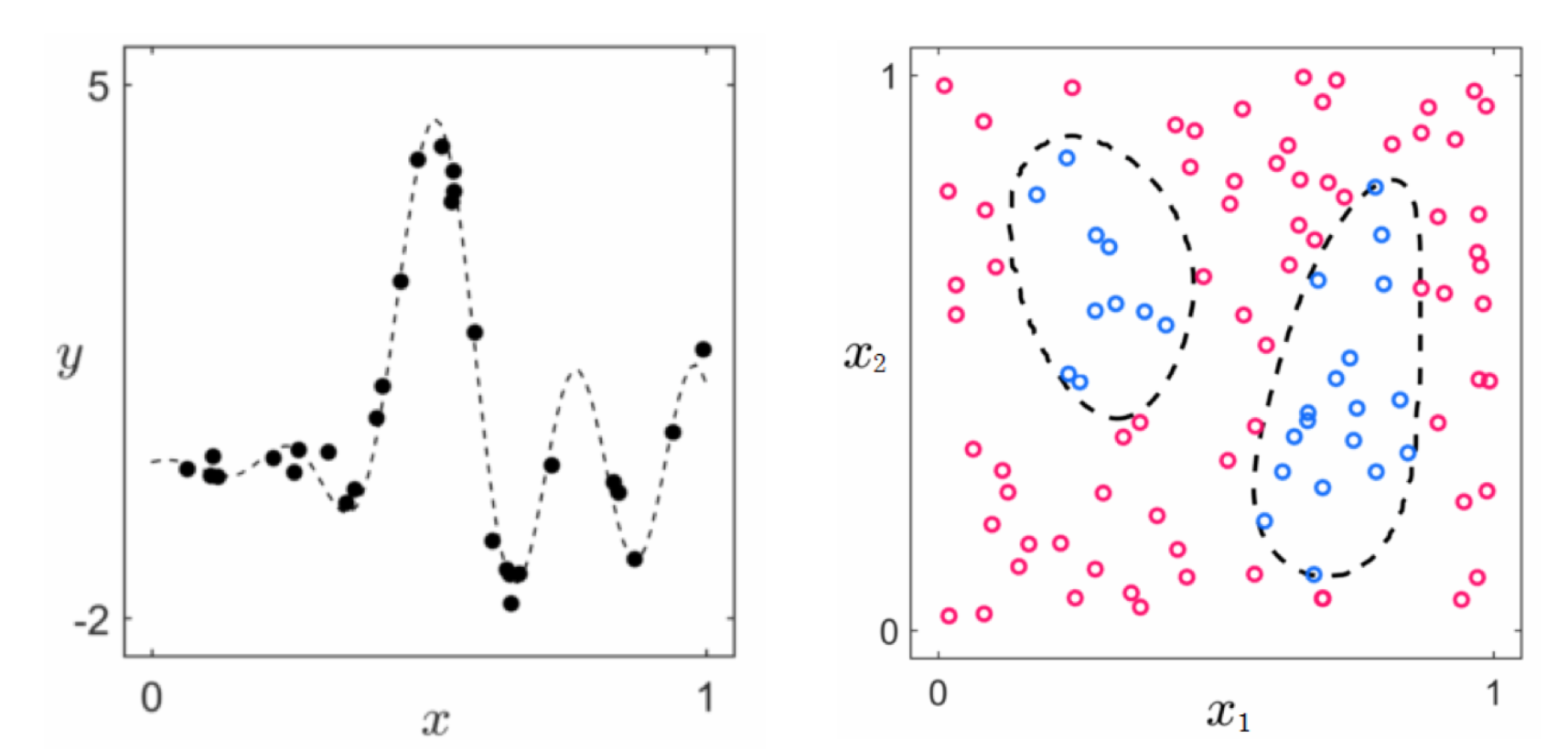
In the previous Sections of this Chapter we saw how to inject arbitrary nonlinear models into both our supervised and unsupervised learning paradigms. However the specific examples we saw illustrating how those principles can be employed were rather simplistic, indeed they were designed specifically so that a proper form of nonlinearity could be determined by visual examination of the data. Of course we cannot rely on our visualization abilities in general - most modern datasets have far more than two inputs which makes visualization impossible. Even in those instances when we can visualize our data it is usually not obvious what sort of explicit nonlinearty(ies) should be used (as with the examples shown in the figure below).

Figure 1: Toy regression (left) and classification (right) datasets that present nonlinear behavior. What specific nonlinear feature transformations would you choose for each dataset? In other words, what sort of specific nonlinearity do you think provides the best nonlinear fit with the regression dataset, and nonlinear separation (a boundary roughly matching the dashed ovoid ones highlighted in the right panel) with the classification data? It is not obvious (at least to us).

However more importantly we do not want to have to identify appropriate nonlinearities ourselves - whether we do this 'by eye' or by our mathematical or philisophical method (i.e., via a differential equations / dynamic systems mindset). With machine learning we want to take the 'easy' way out: we want to automate the process of determining the best nonlinearity(ies) for general datastets.

In machine learning we automate the process of identifying the appropriate nonlinearities / feature transformations for a dataset.

Where do we begin?

The aim to automate nonnlinear learning is an ambitious goal and perhaps - at the start - a seemingly intimidating one. There are an infinite number of nonlinearities to choose from, how do we winnow down these countless choices into a managable, predictable, and user-friendly program? In the next two Sections we introduce the main building blocks of nonlinear automation, called universal approximators and cross-validation.