code

share


In Sections 12.1 - 12.3 we saw how supervised and unsupervised learners alike can be extended to perform nonlinear learning via the use of arbitrary linear combination of nonlinear functions / feature transformations. However the general problem of engineering an appropriate nonlinearity for a given dataset has thus far remained elusive. In this Section we introduce the first of two major tools for handeling this task: universal approximators. Universal approximators are families of simple nonlinear feature transformations whose members can be combined to create artbitrarily complex nonlinearities like any we would ever expect to find in a supervised or unsupervised learning dataset. Here we will also introduce the three standard types of universal approximators employed in practice today - kernels, neural networks, and trees - of which we will have much more to say of in future Chapters.
Virtually every complicated object in the world around us can be decomposed into simpler elements. An automatible consists of components like windows, tires, an engine, and so on. A car engine can be broken down a combination of yet simpler components, into e.g., a set of pistons, an alternator, etc., Even the base alloys used to construct these engine components can be broken down into combinations of metals, and these metals into combinations of elements from the periodic table.
Complicated mathematical objects - i.e., traditional mathematical functions (curves, manifolds, step functions, etc., in general referred to as piecewise-continuous functions) - can be similarly broken down into combinations of simpler elements, i.e., into combinations of simpler mathematical functions. Stated more formally, any (piecewise) continuous mathematical function $h\left(\mathbf{x}\right)$ can be broken down into / approximated by a linear combination of $B$ 'simple' functions $f_1,\,f_2,\,...\,f_B$ in general as
\begin{equation} h\left(\mathbf{x}\right) = w_0 + f_1\left(\mathbf{x}\right){w}_{1} + f_2\left(\mathbf{x}\right){w}_{2} + \cdots + f_B\left(\mathbf{x}\right)w_B \end{equation}where each of the simpler nonlinear functions on the right hand side can have internal parameters. This is actually a rather old mathematical fact (e.g., with roots in the 1700s) which we call universal approximation in the machine learning / deep learning world. These 'simple' functions are called universal approximators. Moreover if we use enough of them, and tune their parameters correctly, we can approximate any function we want.
With enough universal approximators, with correctly tuned parameters, we can approximate any piecewise continuous mathematical function $h\left(\mathbf{x}\right)$ as closely as we wish as $h\left(\mathbf{x}\right) = w_0 + f_1\left(\mathbf{x}\right){w}_{1} + f_2\left(\mathbf{x}\right){w}_{2} + \cdots + f_B\left(\mathbf{x}\right)w_B$
For example, below we show a continuous nonlinear function $h$ in black, and approximate this function using $B = 300$ universal approximators. As you move the slider from left to right you will see a red curve jump onto the screen - this is the combination of our $300$ universal approximators shown first with a poor choice of parameter settings. As yo move the slider from left to right we illustrate how the shape of this combination improves (in terms of how it approximates $h$) as we improve its parameters. Eventually - moving the slider all the way to the right where we show an especially good setting of these parameters - the combination approximates $h$ quite well (and indeed if we kept refining its parameters it could perfectly represent $h$).
Even functions with discrete jumps - like a step function - can be approximated infinitely closely using a combination of universal approximators. Below we show a similar animation to the one above, only there we approximate a step function with nonlinear jumps. Here we use $B=100$ universal approximators, and once again as you move the slider from left to right the parameters of the combination are improved so that the approximation looks more and more like the function $h$ itself.
What are these 'simple' universal approximators $f_1,\,f_2,\,...\,f_B$? How do we set the parameters of this linear combination correctly (including possible internal parameters of the the functions $f_1,\,f_2,\,...\,f_B$)? What does this have to do with determining a proper nonlinearity for a supervised/unsupervised dataset? We address each of these questions below.
There is an enormous variety of 'simple' functions $f_1,\,f_2,\,...\,f_B$ that fall into the category of universal approximators. Typically these are organized into three families or catalogs of similar functions called kernels, neural networks, and trees respectively. Roughly speaking, using functions from any one of these families we can perform the kind of universal approximation described above. That is, using any one of these families we can decompose / approximate any piecewise continuous function as finely as we desire provided we use enough members (i.e., $B$ is large enough) and all parameters are set correctly. Each of these popular families has its own unique strengths and weaknesses, a wide range of technical details to explore, and conventions of usage. Here we introduce them at a high level, but dedicate an entire Chapter to each family in Chapters 13 - 15.
The family of kernel functions consists of groups of functions with no internal parameters, a popular example being polynoimals. When dealing with just one input this sub-family of kernel functions looks like
\begin{equation} f_1(x) = x, ~~ f_2(x) = x^2,~~ f_3(x)=x^3,... \end{equation}and so forth with the $D^{th}$ element taking the form $f_D(x) = x^D$. A combination of the first $D$ units from this sub-family is often referred to as a degree $D$ polynomial. There are an infinite number of these functions - one for each positive whole number - and they are naturally ordered by their degree (the higher the degree, the further down the list that function is). Moreover each element has a fixed shape - e.g., the monomial $f_2(x) = x^2$ is always a parabola, and looks like a cup facing upwards. Below we plot the first four elements (also called units) of the polynomial sub-family of kernel functions.

In two inputs $x_1$ and $x_2$ polynomial units take the analagous form
\begin{equation} f_1(x_1,x_2) = x_1, ~~ f_2(x_1,x_2) = x_2^2, ~~ f(x_1,x_2) = x_1x_2^3, ~~ f(x_1,x_2) = x_1^4x_2^6,... \end{equation}with a general degree $D$ unit taking the form
\begin{equation} f_m(x_1,x_2) = x_1^px_2^q \end{equation}where where $p$ and $q$ are nonnegative integers and $p + q \leq D$. A degree $D$ polynomial in this case is a linear combinatino of all such units. This sort of definition generalizes to defining polynomial units in general $N$ dimensional input as well. Below we draw a sampling of these polynomial units.

Another classic sub-family of kernel universal approximators: sine waves of increasing frequency. This consists of the set of sine waves with frequency increasing by an e.g., integer factor like
$$f_1(x) = \text{sin}(x), ~~ f_2(x) = \text{sin}(2x), ~~ f_3(x) = \text{sin}(3x), ...$$where the $m^{th}$ element given as $f_m(x) = \text{sin}(mx)$.
Below we plot the table of values for the first four of these catalog functions using their equations.

As with the polynomials, notice how each of these catalog of elements if fixed. They have no tunable parameters inside, the third element always looks like $f_3(x) = \text{sin}(x)$ - that is it always takes on that shape. Also note, like polynomials to generalize this catalog of functions to higher dimensional input we shove each coordinate through the single dimensional version of the function separately. So in the case of $N=2$ inputs the functions take the form
\begin{equation} f_1(x_1,x_2) = \text{sin}(x1), ~~ f_1(x_1,x_2) = \text{sin}(2x_1)\text{sin}(5x_2), ~~ f_3(x_1,x_2) = \text{sin}(4x_1)\text{sin}(2x_2), ~~ f_4(x_1,x_2) = \text{sin}(7x_1)\text{sin}(x_2), ~~ ... \end{equation}And these are listed in no particular order, and in general we can write a catalog element as $f_m(x_1,x_2) = \text{sin}(px_1)\text{sin}(qx_2) $ where $p$ and $q$ are any nonnegative integers.
We describe the kernel family in significantly more detail in Chapter 15.
Another family of universal approximators are neural networks. Broadly speaking neural networks consist of parameterized functions whose members - since they are parameterized - can take on a variety of different shapes (unlike kernel functions which each take on a single fixed form). A sub-family of neural networks typically consists of a set of parameterized functions of a single type. For example, a common single layer neural network basis consists of parameterized $\text{tanh}$ functions
\begin{equation} f_1(x) = \text{tanh}\left(w_{1,0} + w_{1,1}x\right), ~~ f_2(x) = \text{tanh}\left(w_{2,0} + w_{2,1}x\right), ~~ f_3(x) = \text{tanh}\left(w_{3,0} + w_{3,1}x\right), ~~ f_4(x) = \text{tanh}\left(w_{4,0} + w_{4,1}x\right), ... \end{equation}Notice that because there are parameters inside the $\text{tanh}$ the $b^{th}$ such function $f_b$ can take on a variety of shapes depending on how we set its internal parameters $w_{b,0}$ and $w_{b,1}$. We illustrate this below by randomly setting these two values and plotting the table of the associated function.

Choosing another elementary function gives another sub-catalog of single-layer neural network functions. The rectified linear unit (or 'relu' for short) is another popular example, elements of which (for single dimensional input) look like
\begin{equation} f_1(x) = \text{max}\left(0,w_{1,0} + w_{1,1}x\right), ~~ f_2(x) = \text{max}\left(0,w_{2,0} + w_{2,1}x\right), ~~ f_3(x) = \text{max}\left(0,w_{3,0} + w_{3,1}x\right), ~~ f_4(x) = \text{max}\left(0,w_{4,0} + w_{4,1}x\right), ... \end{equation}Since these also have internal parameters each can once again take on a variety of shapes. Below we plot $4$ instances of such a function, where in each case its internal parameters have been set at random.

To handle higher dimensional input we simply take a linear combination of the input, passing the result through the nonlinear function. For example, an element $f_j$ for general $N$ dimensional input looks like the following using the relu function
\begin{equation} f_j\left(\mathbf{x}\right) = \text{max}\left(0,w_{j,0} + w_{j,1}x_1 + \cdots + w_{j,\,N}x_N\right). \end{equation}As with the lower dimensional single layer functions, each such function can take on a variety of different shapes based on how we tune its internal parameters. Below we show $4$ instances of such a function with $N=2$ dimensional input.

Other 'deeper' elements of the neural network family are constructed by recursively combining single layer elements. For example, to create a two-layer neural network function we take a linear combination of single layer elements, like the $\text{tanh}$ ones shown above, and pass the result through same $\text{tanh}$ function e.g., summing $10$ elements and passing the result through $\text{tanh}$ gives a 'two-layer' function. With this we have created an even more flexible function, since each internal single-layer function $f_j$ also has internal parameters, which we illustrate by example below. Here we show $4$ random instances of the above neural network function, where in each instance we have randomly set all of its parameters. As can be seen below, these instances are far more flexible than the single-layer ones.
We go into substantially further detail in discussing this family of universal approximators in Chapter 13.

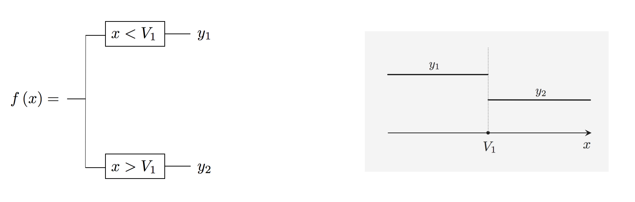
Like neural networks, a single element from the family of tree-based universal approximators can take on a wide array of shapes. The simplest sort of tree basis consists of discrete step functions or, as they are more commonly referred to, stumps whose break lies along a single dimension of the feature space. A stump with 1-dimensional input $x$ can be written as
\begin{equation} f_1(x) = \begin{cases} x < V_1 \,\,\,\,\, a_1 \\ x \geq V_1 \,\,\,\,\, b_1 \end{cases} ~~~~~~~~ f_2(x) = \begin{cases} x < V_2 \,\,\,\,\, a_2 \\ x \geq V_2 \,\,\,\,\, b_2 \end{cases} ~~ \cdots \end{equation}where $V_{1}$ is split point at which the stump changes values, and $y_{1}$ and $y_{2}$ are values taken by the two sides of the stump, respectively, which we refer to as levels of the stump.
Below we plot four instances of such a stump basis element - where we can see how each one takes on a wide variety of shapes.

Higher dimensional stumps follow this one dimensional pattern: a split point $V_1$ is defined along a single dimension, defining a linear step along a single coordinate dimension. Each side of the split is then assigned a single level value. Below we plot four instances of a single stump defined in two dimensions. Here the split point is defined along a value on either the $x_1$ or $x_2$ axis, producing a step that is a line along one coordinate axes.

To create a more flexible decision tree basis function we split each level of the stump. This gives us a tree of depth 2 (our first split gave us a stump, another phrase for stump is tree of depth 1). We can look at this mathematically / figuratively as in the figure below.
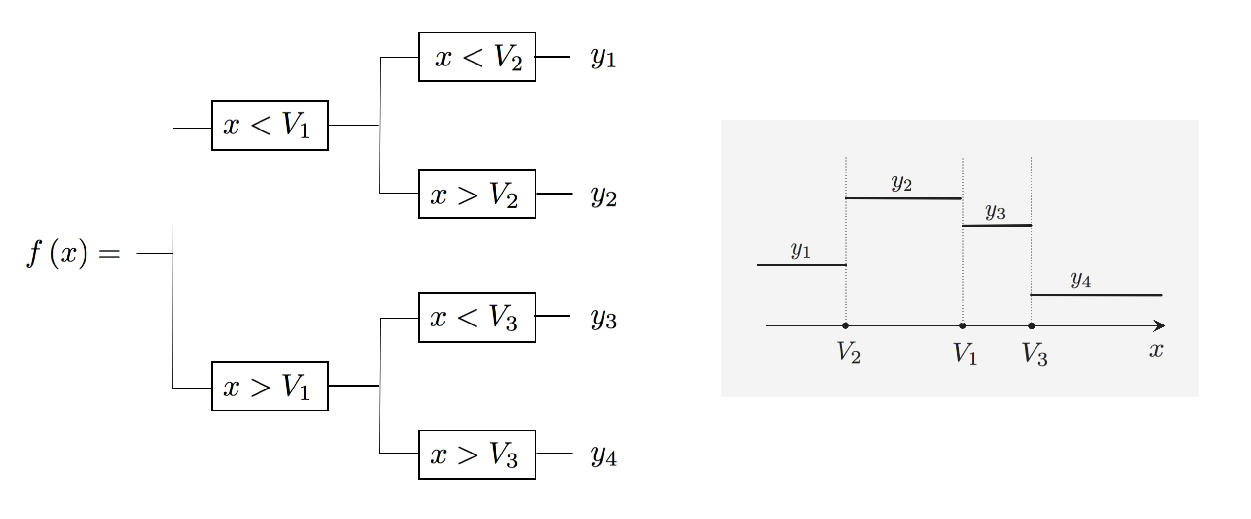
This gives a basis element with four (potentially) distinct levels. Since the location of the splits and the values of the levels can be set in many ways, this gives each element of a tree basis of depth 2 a good deal more flexibility than stumps. Below we illustrate $4$ instances of a depth $2$ tree.
We describe trees in significantly further detail in Chapter 14.

Given a piecewise continuous function $h\left(\mathbf{x}\right)$ and a set of universal approximators parameters approximators $f_1,...,f_B$, how do we best tune the parameters of their linear combination so that - at the very least - we have a good approximation? Stated more formally if we use a linear combination of these approximators as our model
how do we tune all of the parameters in $\mathbf{w}$ - which includes the weights of our linear combination $w_0,\,w_1,...,w_B$ as well as any possible internal parameters of the universal approximators themselves - so that we can at the very least approximate $h\left(\mathbf{x}\right)$ using this linear combination as
\begin{equation} \text{model}\left(\mathbf{x},\mathbf{w}\right) \approx h\left(\mathbf{x}\right). \end{equation}Lets appreciate for a moment just what a general question this is, since we are saying that $h$ can be in general any piecewise continuous function.
As illustrated figuratively below, the aim of correctly tuning parameters in here is actually a case of regression. More specifically, it is an instance of what we call 'perfect' regression - where by 'perfect' we mean that in such a case we have a complete, noise free set of input/output data (the set of points defining the function $h$). For every input point $\mathbf{x}_p$ we have a correpsonding output $y_p = h\left(\mathbf{x}_p\right)$, and so have a very large set of input/output pairs defining the entire function $\left \{\mathbf{x}_p,\, y_p\right\}_{p=1}^P$ (technically $P$ would be infinity, but we can suppose instead that it is just very very large).
So - in other words - to tune the parameters of our model to get the best possible fit to a nonlinear function we can simply minimize a cost function. Here - for the sort of nonlinear functions shown in the figure below - it seems most natural to use a Least Squares of Least Absolute deviations cost.
This indeed how we produced the first animation shown above in Section 12 - the continuous function shown there actually consists of $10,000$ input/output points, and we used $B = 300$ single layer neural network functions with $\text{tanh}$ function (precisely like those detailed in the previous Subsection) to minimize the Least Squares cost
\begin{equation} g\left(\mathbf{w}\right) = \frac{1}{P}\sum_{p=1}^{P}\left(\text{model}\left(\mathbf{x}_p,\mathbf{w}\right) - y_p\right)^2 \end{equation}using gradient descent. Below we re-plot this animation, but show the cost function history plot as well. You can track which weights from the run of gradient descent are currently being used model by a small red dot we have placed on the cost history plot. As yo move the slider from left to right the weights, and overall fit of the model, progress while the red dot on the cost function history traces out which step of the descent run we is currently being shown in the left panel.
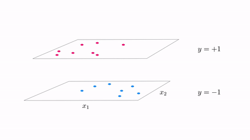
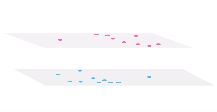
In the same vein our classification cost functions are ideal for tuning hte parameters of a model when the function takes on discrete steps, like the one shown in the second animation in Subsection 12.5.2. There we had a funciton consisting of discrete steps taking on the values $\pm 1$, which we can think of as an example of a 'perfect' case of two-class classification data. Below we illustrate two figurative examples of such 'perfect' classification data - a linear and nonlinear separable dataset. In both cases the 'perfect' dataset consists of a very large, noise free set of data. In the context of classification 'noise' means 'incorrectly labeled', thus if we think about such a 'perfect' classification dataset it is indeed a step function with arbitrary boundary.
Indeed to create the fit shown in the second animation of Subsection 12.5.1 above we tuned the model parameters by minimizing the corresponding softmax cost function
Below we replot this animation, showing the corresponding softmax cost function history along with the animated fit. As with the animation above you can visually track which step of gradient descent is currently being used by the model when you move the slider from left to right by the red dot shown on the cost function history plot.
Another example - this time in three dimensions - is given below. Here we color all points of the function according to our usual coloring scheme for two-class classification: points with output value $+1$ are colored red, while those with output value $-1$ are colored blue. We use the polynomial approximators here, and minimize the softmax cost using Newton's method. In the left panel we view this dataset 'from above', and visualize the learned surface's intersection with the plane $y = 0$ (the decision boundary) as a series of black curves. On the right the data is shown in three dimensions and the learned surface, where the learned surface is given a grid texture so that it is more visually distinct from the function itself. As you pull the slider from left to right the weights used vary from those at the beginning of the run to the end, where the fit is optimal.
The same sort of idea detailed here also holds for multiclass classificaiton as well as unsupervised learning (e.g.,, the nonlinear autoencoder) - their 'perfect' versions are also complete mathematical functions. For all such 'perfect' data - whether it supervised or unsupervised - the moral is this: for 'perfect' data improving the weights of a model consisting of a linear combination of universal approximations by minimizing an associated cost function always improves the model's fit. Likewise, increasing $B$ the number of universal approximators used in a model and properly tuning its parameters always improves the model's fit.
For 'perfect' data improving the weights of a
modelconsisting of a linear combination of universal approximations by minimizing an associated cost function always improves themodel's fit. Likewise, increasing $B$ the number of universal approximators used in amodeland properly tuning its parameters always improves themodel's fit.
This moral holds regardless of the set of universal approximators we choose - whether it be kernels, neural networks, or trees. We illustrate this graphically below using a simple 'perfect' regression dataset, and regress an increasing number of elements or 'units' from each catalog. In the left, middle, and right panels we show the result of fitting an increasing number of polynomial, single layer tanh, and tree units respectively. As you move the slider from left to right you can see the result of fitting more and more of these units, with the result being the same in each instance: we get a better fit to the 'perfect' data.
In reality we virtually never have 'perfect' datasets to learn on, and have to make due with what we have. However the same principal we employ in the 'perfect' data scenario - of employing members of a family of universal approximators in order to uncover the nonlinearity of a dataset - still makes sense here. For example, below we animate the learning of a set of 100 single layer tanh neural network units to a realistic regression dataset that looks something like the first 'perfect' dataset shown in the previous Subsection. Here we show what the resulting fit from $100$ evenly sampled weights from a run of $5000$ gradient descent steps used to minimize the corresponding regression Least Squares cost function. As yo move the slider from left to right you can track which (weights of each) step of gradient descent is being used in the current fit shown by tracking where the red dot on the cost function history plot in the right panel is currently located. As you pull the slider from left to right, using more and more refined weights, the resulting fit gets better.
Below we repeat the experiment above only here we use $50$ stump units, tuning them to the data using $5000$ gradient descent steps. Once again as you move the slider a fit resulting from the certain step of gradient descent reflected on the cost function history is shown, and as you move from left to right the run progresses and the fit gets better.
This same phenomenon holds if we perform any other sort of learning - like classification. Below we use a set of stumps to perform two-class classification, training via gradient descent, on a realistic dataset that is reminiscent of the 'perfect' three dimensional classification dataset shown in the previous Subsection. As you pull the slider from left to right the tree-based model employs weights from further in the optimization run, and the fit gets better.
This sort of trend holds for multiclass classification (and unsupervised learning problems as well), as illustrated in the example below. Here we have tuned $100$ single layer tanh neural network units minimizing the multiclass softmax cost to fit a toy $C=3$ class dataset. As you move the slider below from left to right weights from a run of $10,000$ steps of gradient descent are used, with steps from later in the run used as the slider is moved from left to right.
However there is one very distinct difference between the case of 'perfect' and real data in terms of how we employ universal approximators to correctly determine the proper amount of nonlinearity present in real data: with real data we can tune the parameters of a model employing universal approximators too well, and/or use too many of universal approximators, and/or use universal approximators that are too nonlinear for the dataset given. In short, the model we use (a linear combination of universal approximators) can be too nonlinear for a real dataset.
For example, below we animate the fit provided by a large number of polynomial units to the real regression dataset shown in the first two examples of this Subsection. Here we progressively fit more and more polynomial units to this dataset, displaying the resulting fit and corresponding Least Squares error provided by the nonlinear model. As you move the slider from left to right you can see the result of fitting each successive polynomial model to the dataset, with the number of polynomials in the model shown displayed over the left panel (where the data and corresponding fit are shown). In the right panel we show the Least squares error - or cost function value - of this model. As you can see moving the slider from left to right, adding more polynomial units always decreases the cost function value (just as in the 'perfect' data case) however the resulting fit - after a certain point - actually gets worse. It is not that the model is fitting the training data worse as the model becomes more flexible, it is simply that after a certain number of universal approximators are used (here around 15) the tuned model clearly becomes too nonlinear for the phenomenon at hand, and hence becomes a poor model for future test data.
This sort of phenomenon is a problem regardless of the sort of universal approximator we use - whether it be a kernel, neural network, or tree-based catalog of functions. As another example, below we animate the fitting of $1$ through $20$ polynomials (left panel), single layer tanh neural network (middle panel), and stump units (right panel) to the simple sinusoidal regression dataset we have used previously in e.g., the first example in Section 12.1. As you move the slider from left to right you will see the fit resulting from the use of more and more of each type of unit. As you continue to add units in each case the resulting fit indeed provides a better fit to the training data, but after a certain point for each type of universal approximator the fit clearly becomes poor for future test data.
This same problem presents itself with all real supervised / unsupervised learning datasets. For example, if we take the two-class classification dataset shown in the third example of this Subsection and more completely tune the parameters of the same set of stumps we learn a model that - while fitting the training data we currently have even better than before - is far too flexible for future test data. Moving the slider one knotch to the right shows the result of a (nearly completely) optimized set of stumps trained to this dataset - with the resulting fit being extremely nonlinear (far to nonlinear for the phenomenon at hand).
As with regression, this sort of phenomenon can happen irregardless of the sort of universal approximator we use. For example, below we show the subsequent fitting of a few degree $D$ polynomials in the range between $1$ through and $50$ to the same dataset. While the cost function value / fit to the training data indeed decreases with each subsequent polynomial, as you can see - after a certain point - the fit becomes far too nonlinear.
In the jargon of machine learning / deep learning the amount of nonlinearity, or nonlinear potential, a model has is commonly referred to as the model's capacity. With real data in practice we need to make sure our trained model does not have too little capacity (it is not too rigid) nor too much capacity (that it is not too flexible). In the jargon of our trade this desire - to get the capacity just right - often goes by the name the bias-variance trade-off. A model with too little capacity is said to underfit the data, or to have high bias. Conversely, a model with too much capacity is said to overfit the data, or have high variance.
Phrasing our pursuit in these terms, this means that with real data we want to tune the capacity of our model 'just right' as to solve this bias-variance trade-off, i.e., so that our model has neither too little capacity (a 'high bias' or underfitting) nor too much capacity (a 'high variance' or overfitting).
With real data in practice we need to make sure our
modeldoes not have too little capacity (it is not too rigid) nor too much capacity (that it is not too flexible). In the jargon of our trade this desire - to get the capacity of ourmodeljust right - often goes by the name the bias-variance trade-off. Amodelwith too little capacity is said to underfit the data, or to have high bias. Conversely, amodelwith too much capacity is said to overfit the data, or have high variance.
With perfect data - where we have (close to) infinitely many training data points that perfectly describe a phenomenon - we have seen that we can always determinine appropriate nonlinearity by increasing the capacity of our model. By doing this we consistently decreases the error of the model on this training dataset - while improving how the model represents the (training) data.
However with real data we saw that the situation is more sensitive. It is still true that by increasing a model's capacity we decrease its error on the training data, and this does improve its ability to represent our training data. But because our training data is not perfect - we usually have only a subsample of (noisy examples of) the true pheenomenon - this becomes problematic when the model begins overfitting. At a certain point of capacity the model starts representing our training data too well, and becomes a prediction tool for future input.
The problem here is that nothing about the training error tells us when a model begins to overfit a training dataset. The phenomenon of overfitting is not reflected in the training error measurment. So - in other words - training error is the wrong measurment tool for determining the proper capacity of a model. If we are searching through a set of models, in search of the one with very best amount of capacity (when properly tuned) for a given dataset, we cannot determine which one is 'best' by relying on training error. We need a different measurement tool to help us determine the proper amount of nonlinearity a model should have with real data.
Notice in the examples here, when constructing a model with universal approximator feature transformations we always use a single kind of universal approximator per model. That is, we do not mix exemplars from different univeral approximator families - using e.g., a few polynomial units and a few tree units in the same model. This is done for several reasons. First and foremost - as we will see in Chapters following this one (with one Chapter dedicated to additional technical details relating to each universal approximator family) - by restricting a model's feature transforms to a single family we can (in each of the three cases) better manage our search for a model with the proper capacity for a given dataset, optimize the learning process, and better deal with each families' unique eccentricities.
However it is quite common place to learn a set of models - each employing a single family of universal approximators - to a dataset, and then combine or ensemble the fully trained models. We will discuss this further later on in this Chapter.