code

share


Unlike polynomials and other fixed kernels, each unit of a neural network has internal parameters that can be tuned to give it a flexible shape. In this Section we detail multi-layer neural networks - often called multi-layer perceptrons or deep feedforward neural networks. In the previous Chapter we introduced single layer perceptrons, and here we expand on that introduction extensively. We will see how these recursively defined universal approximators are defined mathematically as well as implemented (as a feature_transforms function) that we can employ for any supervised or unsupervised learning task we wish.
We begin by describing deep networks in the context of our previous discussion, as a particular catalog of nonlinear functions used for nonlinear learning problems. Along the way we will describe these network elements from a graphical, algebraic, and computational perspective (implementing them as our feature_transforms function) so that we can better understand them.
At the heart of nonlinear learning is the following simple yet powerful idea: nonlinear curves of arbitrary shape can be modeled/approximated via a linear combination of simpler nonlinear functions (or units) of the input data. With neural networks each of these units is also parameterized with a number of weights to be tuned using data. Here we discuss in detail how to form neural network units starting with the simplest of them: a single-layer unit. These are also often referred to as single hidden layer perceptrons as well.
Ever since Hippocrates argued, over two thousand years ago, that the brain was "the seat of the mind," scientists have been studying it with the hope of unlocking the secrets of human intelligence. In fact the field we know today as Artificial Intelligence (AI) was born in an ambitious quest to mathematically model the complex human brain. The first attempts were made in the 1940s [1,2] by a group of psychologists and neuroscientists who proposed simplistic mathematical models for a single neuron (brain cell). These early models - later dubbed as artificial neurons - culminated in the introduction of the perceptron model [3] in 1957.
Figure 1 shows a comparative illustration of a biological neuron (left) and a perceptron (right). The biological neuron consists of three main parts: dendrites (the neuron's receivers), soma (the cell body), and axon (the neuron's transmitter). Closely mimicking this structure, an artificial neuron comprises a set of dendrite-like edges, each taking an input and multiplying it by a (synaptic) weight associated with that edge. These weighted inputs are summed up after going through a summation unit (shown in the figure by a small hollow circle). The result is subsequently fed to an activation unit (shown by a large blue circle) whose output is then transmitted to the outside via an axon-like projection. Notice how the output of the perceptron model takes the same form as a single-layer basis function derived in Subsection 1.1.1. The graphical model shown in the right panel of Figure 1 is therefore commonly used to visually represent a single-layer neural network basis function.
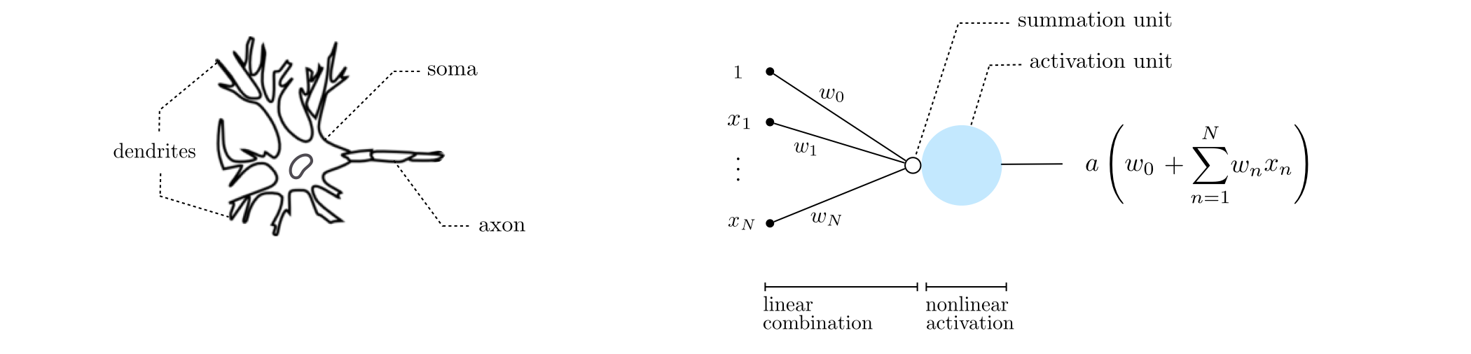
From a biological perspective, neurons are believed to remain inactive until the net input to the cell body (soma) reaches a certain threshold, at which point the neuron gets activated and fires an electro-chemical signal, hence the name activation function.
The algebraic representation of the sort of single-layer unit function shown in the Figure above is quite simple: a linear combination of the input passed through a nonlinear activation function
\begin{equation} f^{(1)}\left(\mathbf{x}\right)=a\left(w^{\left(1\right)}_{0}+\underset{n=1}{\overset{N}{\sum}}{w^{\left(1\right)}_{n}\,x_n}\right). \end{equation}The superscripts on $f$ and $w_0, w_1, \ldots, w_N$ indicate they represent a single-layer function and its internal weights respectively. Because we will want to extend the single layer idea to create deeper - multilayer - perceptrons, we will find that it is easier to describe this sort of function as a sequence of two operations: the linear combination of input, passed through a nonlinear activation. We refer to this manner of writing out the function as the recursive recipe for creating single layer perceptron units and show it below.
1: input: Activation function $a\left(\cdot\right)$
2: Compute linear combination: $\,\,\,\,\,\,\,\,\, v = w_{0}^{(1)}+{\sum_{n=1}^{N}}{w_{n}^{(1)}\,x_n}$
3: Pass result through activation: $\,\,\, a\left(v\right)$
4: output: Single layer unit $\,\, a\left(v\right)$
In the Python cell below we plot four instances of a single-layer unit using $\text{tanh}$ as nonlinear activation function. These take the form
\begin{equation} f^{(1)}(x) = \text{tanh}\left(w_0^{(1)} + w_1^{(1)}x\right) \end{equation}In each instance the internal parameters have been set randomly, giving each basis function a distinct shape.

We repeat the experiment in Example 1, this time swapping $\text{tanh}$ for ReLU as activation, i.e., they take the form
\begin{equation} f^{(1)}(x) = \text{max}\left(0,w_0^{(1)} + w_1^{(1)}x\right) \end{equation}In each instance the internal parameters have been set randomly, giving each basis function a distinct shape.

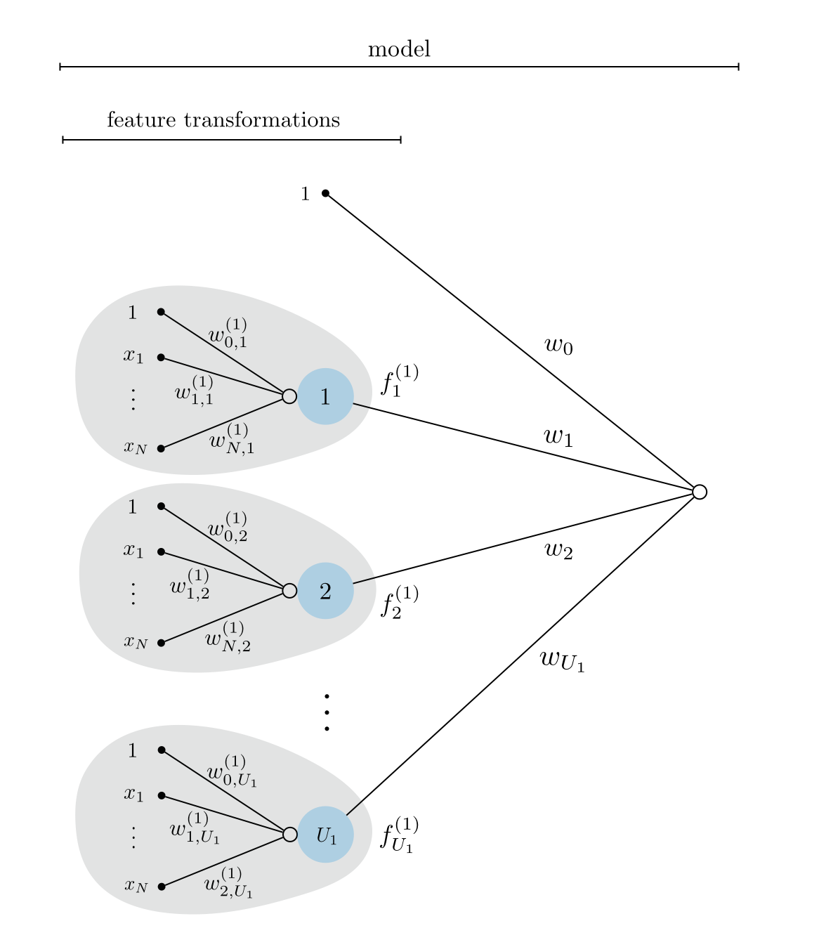
In general we will want to compute $B = U_1$ such units - a number we define - as feature transformations in supervised / unsupervised learning model
as we described in the previous Chapter where we introduced the idea of nonlinear learning. Notice in this case that each single layer unit now has its own internal parameters, the $j^{th}$ of which looks like
\begin{equation} f^{(1)}_j\left(\mathbf{x}\right)=a\left(w^{\left(1\right)}_{0,\,j}+\underset{n=1}{\overset{N}{\sum}}{w^{\left(1\right)}_{n,\,j}\,x_n}\right). \end{equation}These are our feature transformations, which we implement in a feature_transforms module (as done repeatedly in Chapter 12) in the next Subsection. Figure 2 shows a graphical representation of these feature transformations along with their linear combination - a single layer neural network model whose algebraic form is given in (4).
Pythonic implementation of single layer units¶Because our ultimate goal is to implement our single layer units in a feature_transforms function, it is first helpful - in terms of producing effecient Python code - to write all $U_1$ of these functions together using more compact mathematical notation. This notation helps us avoid explicit for loops and leverages the Numpy library for effecient array computations. To do this we first employ our standard compact notation where we place a $1$ at the top of our input $\mathbf{x}$, which denote by placing the $\mathring{}$ symbol over this notation as
Next we collect all of the internal parameters of our $U_1$ single layer units - examining the algebraic form for the $j^{th}$ unit above, we can see that it has $N+1$ internal parameters. Taking these parameters we form a $(N+1) \times 1$ column vector - starting with the bias $w^{\left(1\right)}_{0,\,j}$, and then input-touching weights $w^{\left(1\right)}_{1,\,j}$ through $w^{\left(1\right)}_{N,\,j}$ - and place them into the $j^{th}$ column of a $(N+1) \times U_1$ matrix $\mathbf{W}_1$
\begin{equation} \mathbf{W}_{1}=\left[\begin{array}{cccc} w_{0,1}^{\left(1\right)} & w_{0,2}^{\left(1\right)} & \cdots & w_{0,U_{1}}^{\left(1\right)}\\ w_{1,1}^{\left(1\right)} & w_{1,2}^{\left(1\right)} & \cdots & w_{1,U_{1}}^{\left(1\right)}\\ \vdots & \vdots & \ddots & \vdots\\ w_{N,1}^{\left(1\right)} & w_{N,2}^{\left(1\right)} & \cdots & w_{N,U_{1}}^{\left(1\right)} \end{array}\right]. \end{equation}With this notation note how the matrix-vector product $\mathbf{W}_{1}^T\,\mathbf{x}$ contains every linear combination internal to our $U_1$ units. In other words, it has dimensions $U_1 \times 1$, and its $j^{th}$ entry is precisely the linear combination of the input data internal to the $j^{th}$ unit as
\begin{equation} \left(\mathbf{W}_{1}^T\,\mathring{\mathbf{x}}\right)_j = w^{\left(1\right)}_{0,\,j}+\underset{n=1}{\overset{N}{\sum}}{w^{\left(1\right)}_{n,\,j}\,x_n} \,\,\,\,\,\,\,\,\,\,\,\,\,\,\, j=1,...,U_1. \end{equation}Then we extend our notation for the activation function $a\left(\cdot\right)$ to handle such a vector. More specifically we define $\mathbf{a}$ as the vector function that takes in a general $d \times 1$ vector $\mathbf{v}$ and returns as activation of each of its entries
\begin{equation} \mathbf{a}\left(\mathbf{v}\right)=\left[\begin{array}{c} a\left(v_{1}\right)\\ \vdots\\ a\left(v_{d}\right) \end{array}\right]. \end{equation}Now note how - with this notation - the vector-activation of the matrix-vector product $\mathbf{a}\left(\mathbf{W}_{1}^T\,\mathring{\mathbf{x}}\right)$ is a $U_1 \times 1$ vector contains all $U_1$ single layer units as
\begin{array} \ \mathbf{a}\left(\mathbf{W}_{1}^T\,\mathring{\mathbf{x}}\right)_j = a\left(w^{\left(1\right)}_{0,\,j}+\underset{n=1}{\overset{N}{\sum}}{w^{\left(1\right)}_{n,\,j}\,x_n^{\,}}\right) \,\,\,\,\,\,\,\,\,\,\,\,\,\,\, j=1,...,U_1. \\ \end{array}At times when it is convenient we will also use the notation $\mathbf{f}^{(1)}$ to denote this compact set of all $U_1$ of our single layer units
\begin{equation} \mathbf{f}^{(1)} = \mathbf{a}\left(\mathbf{W}_{1}^T\,\mathring{\mathbf{x}}\right). \end{equation}Now we can construct our entire set of $U_1$ single layer perceptron units very efficiently (leveraging Numpy's effecient matrix-vector product computation) as a feature_transforms function that takes in x - our input data - and the correctly sized matrix $\mathbf{W}_1$ - denoted as W_1. We show such an implementation below. Here we use the example of tanh as our activation function, but this is easily swapped out for any other.
# an example activation function - tanh
def activation(v):
    return np.tanh(v)

# a feature_transforms function for computing
# U_1 single layer perceptron units efficiently
def feature_transforms(x, W_1):
    #  pad with ones (to compactly take care of bias) for first layer computation
    o = np.ones((1,np.shape(x)[1]))
    x = np.vstack((o,x))

    # compute linear combination of current layer units
    v = np.dot(x.T, W_1).T

    # pass through activation
    a = activation(v)
    return a
With our feature transforamtions function complete we can use precisely the same formm of model implementation we employed in the previous Chapter, which we repeat below for convenience.
Here our inputs to this Python function are x - our input data - and a list of length two whose first entry contains our matrix of weights $\mathbf{W}_1$ as w[0] = W_1 and whose second entry contains the $U_1 + 1$ weights linear combination weights $w_0,...,w_{U_1}$ packaged as a $\left(U_1 + 1\right) \times 1$ array in w[1].
# an implementation of our model employing a nonlinear feature transformation
def model(x,w):
    # feature transformation
    f = feature_transforms(x,w[0])

    # tack a 1 onto the top of each input point all at once
    o = np.ones((1,np.shape(f)[1]))
    f = np.vstack((o,f))

    # compute linear combination and return
    a = np.dot(f.T,w[1])
    return a.T
Before we look at a few examples, note that we can express our model using the sort of compact notation we employed in writing our set of single layer units so effectively. Using a notation to denote the weights of the linear combination as
and extend our vector $\mathbf{f}^{(1)}$ by tacking a $1$ on top of it - which as usual we denote by adding a $\mathring{}$ symbol to the top of notation as $\mathring{\mathbf{f}}^{(1)}$ - we can then write out the model in equation (4) quite compactly as
\begin{equation} \text{model}\left(\mathbf{x},\mathbf{w}\right) = \mathbf{w}_2^T\mathring{\mathbf{f}}^{(1)}=\mathbf{w}_2^T\mathring{\mathbf{a}}\left(\mathbf{W}_{1}^T\,\mathring{\mathbf{x}}\right) \end{equation}where we use the notation $\mathbf{w}$ on the left hand side to denote all of the weights on the right - i.e., both $\mathbf{w}_2$ and $\mathbf{W}_1$. Note on the right hand side we have also placed a $1$ at the top of $\mathbf{a}$.
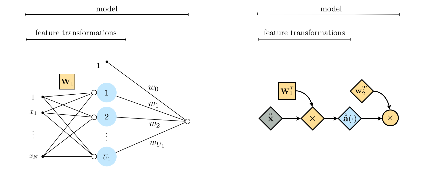
Using the definition of $\mathbf{W}_1$ in Equation (7), in the left panel of Figure 3 we illustrate a more compact but equivalent representation of the single-layer neural network shown originally in Figure 2, where all the internal weights of the feature transformations are now stored in the matrix $\mathbf{W}_1$. Further using our condensed notation in the right panel of Figure 3 we show an even more compact representation of a single-layer neural network via its so-called computational graph, wherein scalars, vectors, and matrices are depicted symbolically as circles, diamonds, and squares, respectively.
Here we repeat a nonlinear regression first shown in Section 12.5 using the dataset shown below, but employing the feature_transforms function developed above for single layer units.

Here we use $U_1 = 100$ units, the tanh activation, and make a run of $5,000$ steps of gradient descent with $\alpha = 10^{-1}$ to fit all of model parameters. Note that in order to initialize our model we need to create a list whose first entry contains the weights of our final linear combination, and whose second entry contains our array of internal weights - which we show below.
# define the number fo units to use
U_1 = 100     # number of single layer units to employ
N = 1         # dimension of input

# initialize internal weights of our single layer units
W_1 = 0.1*np.random.randn(N+1,U_1)

# initialize weights of our linear combination
w_2 = 0.1*np.random.randn(U_1+1,N)

# package weights together
w = [W_1,w_2]
With our run complete can then plot the resulting fit to the data, as shown below, which fits the data quite well.

In this example we learn a nonlinear manifold for the dataset shown below using an encoder and decoder models, each consisting of $U_1 = 10$ single layer tanh units. To see how both encoding/decoding schemes mimic our model functionality see Section 12.4, where the notion of a nonlinear encoder was introduced.

Using our feature_transforms function for both encoding and decoding functions we make a run of $1,000$ steps of gradient descent with $\alpha = 10^{-1}$ to fit all of autoencoder's parameters. Note that in order to initialize our model we need to create a list whose first entry contains the weights of our final linear combination, and whose second entry contains our array of internal weights - for each of the encoding and decoding functions precisely as we did in the previous example.
With our run complete can then plot the resulting nonlinear manifold fit to the data, as shown below, which represents the data quite well. In the bottom panel we illustrate how - once trained - the points in this space gravitate towards the learned autoencoder.


That single-layer units we discussed above have tunable internal parameters, giving them a range of possible shapes to take as saw in Examples 1 and 2. However, the flexibility of each unit is limited to some extent. In Example 1 all we can control is the horizontal placement of the function (via $w_{0}$) and the steepness of the transition from $-1$ to $1$ (via $w_{1}$). Similarly in Example 2, we can only move the ReLU in the horizontal direction and change the slope of its forearm.
We boost the flexibility (or capacity) of these units by creating deeper two layer perceptrons, as we now describe. These are also often referred to as two hidden layer perceptrons as well.
To create a two-layer perceptron unit we recurse on the idea of a single layer unit. In short, to create a two layer unit we first construct a set of $U_1$ single layer units and treat them as we treated the input: that is we take their linear combination and pass the result through a nonlinear activation. This idea is illustrated graphically in Figure 4 below.
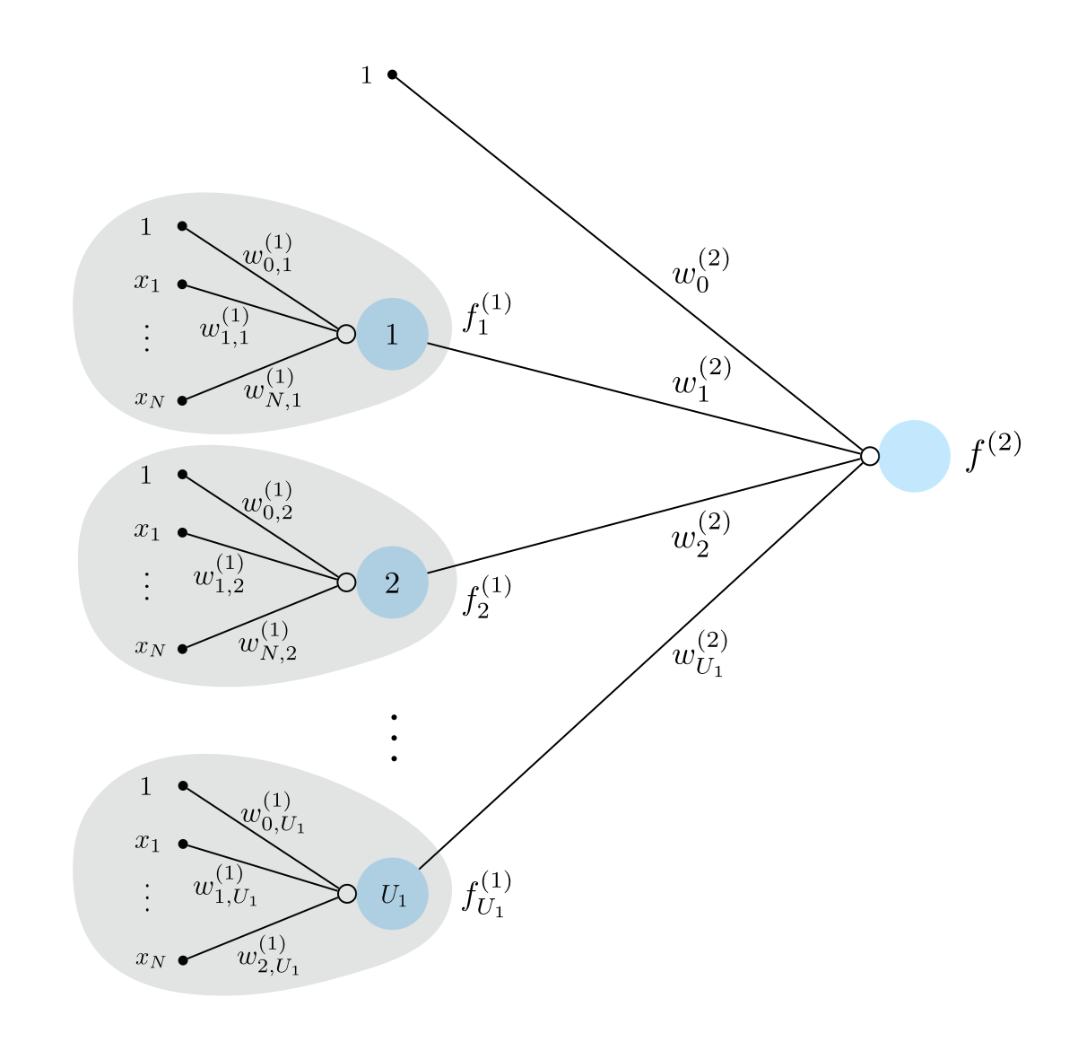
If we were to write out the algebraic form of a two-layer unit shown in the Figure above $f^{\left(2\right)}\left(\mathbf{x}\right)$ we have the formula
\begin{equation} f^{\left(2\right)}\left(\mathbf{x}\right)=a\left(w^{\left(2\right)}_{0}+\underset{i=1}{\overset{U_1}{\sum}}{w^{\left(2\right)}_{i}}\,f^{(1)}_i\left(\mathbf{x}\right)\right) \end{equation}which reflects the recursive nature of the second layer unit algebraically. As was the case with the single layer unit, this formula is perhaps easier to digest if we think about each step of the computation starting from the most internal (that is, the construction of the first layer units) to the final outer activation function. We detail pulled-apart way of expressing the generic two layer unit algebraically in the 'recursive recipe' below.
1: input: Activation function $a\left(\cdot\right)$, number of single layer units $U_1$
2: Construct single layer units: $\,\,\,\,\,\,\,\,\,f^{(1)}_i\left(\mathbf{x}\right)$ for $i=1,\,...,U_1$
3: Compute linear combination: $\,\,\,\,\,\,\, v = w_{0}^{(2)}+{\sum_{i=1}^{U_1}}{w_{i}^{(2)}\,f^{(1)}_i}\left(\mathbf{x}\right)$
4: Pass result through activation: $\,\,\,\, a\left(v\right)$
5: output: Two layer unit $\,\, a\left(v\right)$
We plot four instances of a two-layer function using $\text{tanh}$ as activation, akin to what we did in Example 1. All weights are again set randomly in each instance. These look like
\begin{equation} f^{(2)}(x) = \text{tanh}\left(w_0^{(2)} + w_1^{(2)}\,f^{(1)}(x)\right) \end{equation}where
\begin{equation} f^{(1)}(x) = \text{tanh}\left(w_0^{(1)} + w_1^{(1)}x\right) \end{equation}Because this second layer unit has more internal parameters, consisting of linear combinations of single layer units, it is more flexible than the single layer units themselves.

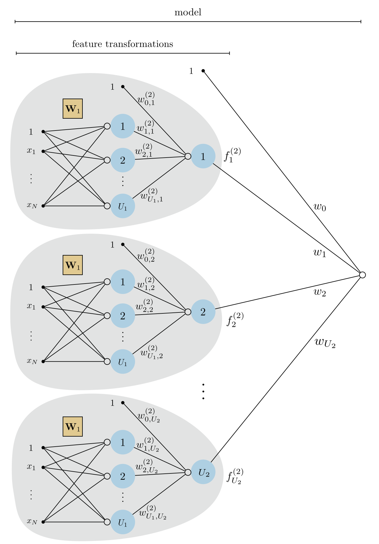
In general we will want to compute $B = U_2$ such two layer units - a number we define - as feature transformations in supervised / unsupervised learning model
as we described in the previous Chapter where we introduced the idea of nonlinear learning. Notice in this case that each two layer unit now has its own unique internal parameters in the linear combination of single layer units (but the weights intnernal to the single layer units are the same for each two layer unit we define). The $j^{th}$ of which looks like
\begin{equation} f^{\left(2\right)}_j\left(\mathbf{x}\right)=a\left(w^{\left(2\right)}_{0.j}+\underset{i=1}{\overset{U_1}{\sum}}{w^{\left(2\right)}_{i,j}}\,f^{(1)}_i\left(\mathbf{x}\right)\right) \end{equation}These are our feature transformations, which we implement in a feature_transforms module (as done repeatedly in Chapter 12) as follows.
Figure 5 shows a graphical representation of these feature transformations along with their linear combination - a two-layer neural network model whose algebraic form is given in (16).
Pythonic implementation of two layer units¶To construct an effecient feature_transforms function employing our two layer units we will use the same sort of compact notation - which carries over nicely in Python - used previously to implement single layer units in the previous Subsection. There we commpactly represented our $U_1$ single layer units using the notation as
(see the previous Subsection for a description of this notation). Following the same pattern here to compactly express our second layer units, we first put all of the internal weights from $U_2$ functions. Note how since the $j^{th}$ second layer unit's input are our $U_1$ first layer units, there are are $U_1 + 1$ internal weights: the bias $w^{\left(2\right)}_{0.j}$ and then input-touching weights $w^{\left(2\right)}_{1,j}$ through $w^{\left(2\right)}_{U_1,j}$. Stacking these weights into the $j^{th}$ column of a matrix $\mathbf{W}_2$ then gives us a $\left(U_1 +1 \right)\times U_2$ matrix of all our units' internal weights
\begin{equation} \mathbf{W}_{2}=\left[\begin{array}{cccc} w_{0,1}^{\left(2\right)} & w_{0,2}^{\left(2\right)} & \cdots & w_{0,U_{2}}^{\left(2\right)}\\ w_{1,1}^{\left(2\right)} & w_{1,2}^{\left(2\right)} & \cdots & w_{1,U_{2}}^{\left(2\right)}\\ \vdots & \vdots & \ddots & \vdots\\ w_{U_1,1}^{\left(2\right)} & w_{U_1,2}^{\left(2\right)} & \cdots & w_{U_1,U_{2}}^{\left(2\right)} \end{array}\right] \end{equation}which mirrors precisely how we defined the $\left(N+1\right) \times U_1$ internal weight matrix $\mathbf{W}_1$ for our single layer units.
With this compact matrix notation we can then express all $U_2$ of our second layer units simulataneously in a single recursive vector-matrix computation
Notice - in comparing the formula above to the one given for the single layer units in equation (18) - how our recursive definition of the two layer units is beautifully reflected in this compact notation. Also if we unwravel our notation our two layer units can also be written as $\mathbf{f}^{(2)} = \mathbf{a}\left(\mathbf{W}_2^T\mathring{\mathbf{a}}\left(\mathbf{W}_{1}^T\,\mathring{\mathbf{x}}\right)\right)$. In either case, we do indeed have that the $j^{th}$ element of this computation is our $j^{th}$ second layer unit
\begin{equation} \mathbf{f}^{(2)}_j = f^{\left(2\right)}_j\left(\mathbf{x}\right). \end{equation}Now we can construct our entire set of $U_2$ two layer perceptron units very efficiently (leveraging Numpy's effecient matrix-vector product computation) as a feature_transforms function that takes in x - our input data - and the correctly sized matrix $\mathbf{W}_1$ for our first layer units and $\mathbf{W}_2$ for our second layer units - which we will input into the function as a list of matrices
w = [W_1,W_2].
Such a list of matrices or arrays is often called a tensor.
In any case, below we provide an implementation based on the notation above for computing all of our $U_2$ second layer units effectively. Notice how this two layer function matches structurally the single unit implementation given previously, but now we must loop over our tensor of matrices: on the first loop we compute all single layer units, and on the second we compute our second layer units.
# a feature_transforms function for computing
# U_2 two layer perceptron units efficiently
def feature_transforms(x, w):
    # assign new name to input x for recursive loop
    a = x

    # loop through each layer matrix
    for W in w:
        # pad with ones (to compactly take care of bias) for
        # current layer computation
        o = np.ones((1,np.shape(a)[1]))
        a = np.vstack((o,a))

        # compute linear combination of current layer units
        v = np.dot(a.T, W).T

        # pass through activation
        a = activation(v)
    return a
Before we look at a few examples, note that we can express our model using the sort of compact notation we employed in writing our set of two layer units so effectively. Using a notation to denote the weights of the linear combination as
and extend our vector $\mathbf{f}^{(2)}$ by tacking a $1$ on top of it - which as usual we denote by adding a $\mathring{}$ symbol to the top of notation as $\mathring{\mathbf{f}}^{(2)}$ - we can then write out the model in equation (16) quite compactly as
\begin{equation} \text{model}\left(\mathbf{x},\mathbf{w}\right) = \mathbf{w}_3^T\mathring{\mathbf{f}}^{(2)} \end{equation}where we use the notation $\mathbf{w}$ on the left hand side to denote all of the weights on the right - i.e., $\mathbf{w}_3$, $\mathbf{W}_2$, and $\mathbf{W}_1$.
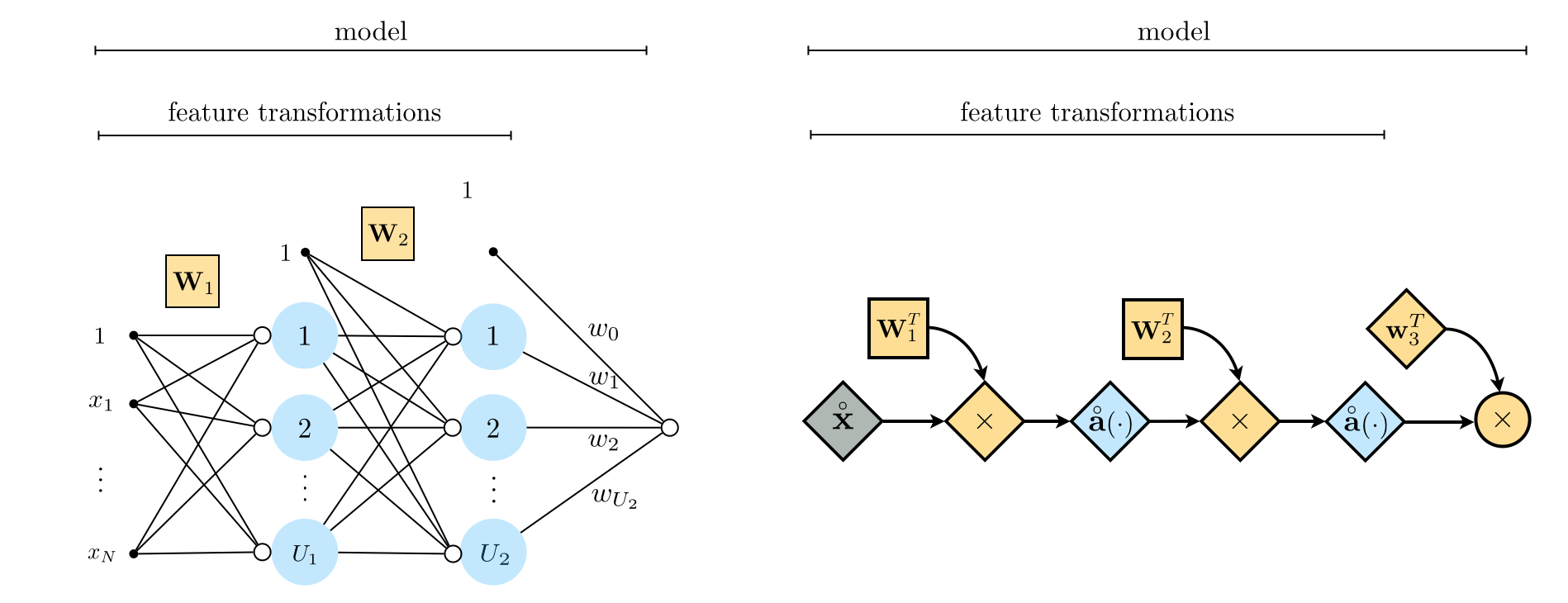
In the left panel of Figure 6 below we show a more compact representation of a two-layer network, employing the matrix notation defined in (19). Further using our condensed notation in the right panel we show its associated computational graph.
In this examople we will employ the two layer unit feature_transforms function above to perform nonlinear multiclass classification using the dataset shown below.

Here we chose the number of units $U_1$ and second units $U_2$ at random as $U_1 = 12$ and $U_2 = 5$. Here we will use $10,000$ gradient descent steps to tune all of the parameters of our model: the weight matrices $\mathbf{W}_1$ and $\mathbf{W}_2$, along with our linear combination weights $\mathbf{w}_3$. Below we show how to initialize the entire set of parameters for our model. Notice here since we are performing $C=3$ class classification that - as discussed in Chapter 10 - we actually employing $3$ models, and so have $3$ sets of final linear combination weights. We initialize and package them all together below by setting w_3 = 0.1*np.random.randn(U_2+1,3).
# define the number fo units to use in each layer
N = 2         # dimension of input
U_1 = 12      # number of single layer units to employ
U_2 = 5       # number of two layer units to employ

# initialize internal weights of our single layer units
W_1 = 0.1*np.random.randn(N+1,U_1)

# initialize internal weights of our second layer units
W_2 = 0.1*np.random.randn(U_1+1,U_2)

# initialize weights of our linear combination
w_3 = 0.1*np.random.randn(U_2+1,3)

# package all weights together in a single list
w = [W_1,W_2,w_3]
Now we make our run of gradient descent, taking $10,000$ steps with $\alpha = 10^{-1}$, to minimize the multiclass softmax cost employing our feature_transforms function and the initialization above. We plot out the cost / misclassification history from this run below to verify that our models have been well tuned. As can be seen below, after a few thousand iterations we achieve perfect classification results.

Now we plot the resulting fit, visualizing the surface fit and - simultaneously - the nonilnear boundary from our best set of weights below.

By recursing on the pattern we have seen above in describing single and two layer perceptron units we can construct arbitrary multilayer perceptron units, likeiwse called deep networks. Here we extend the discussion above in order to achieve this generality, constructing $L$ layer multilayer perceptrons.
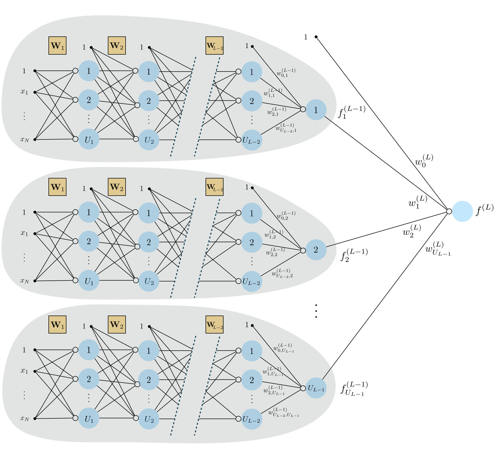
In Figure 7 below we show the graphical representation of a general $L$ layer multilayer perceptron unit. To construct a perceptron like this with an arbitrary number of layers we simply recurse on the pattern we have seen established for single- and two-layer units above. In other words, to construct such a unit we take a linear combination of $L-1$ layer units and pass the result through an activation.
If we were to write out the algebraic form of an $L$ layer unit shown in the Figure above $f^{\left(L\right)}\left(\mathbf{x}\right)$ we have the formula
\begin{equation} f^{\left(L\right)}\left(\mathbf{x}\right)=a\left(w^{\left(L\right)}_{0}+\underset{i=1}{\overset{U_{L-1}}{\sum}}{w^{\left(L\right)}_{i}}\,f^{(L-1)}_i\left(\mathbf{x}\right)\right). \end{equation}which reflects the recursive nature of the $L$ layer unit algebraically. As was the case with the two layer unit, this formula is perhaps easier to digest if we think about each step of the computation starting from the most internal (that is, the construction of the first layer units) to the final outer activation function. We detail pulled-apart way of expressing the generic two layer unit algebraically in the 'recursive recipe' below.
1: input: Activation function $a\left(\cdot\right)$, number of single layer units $U_1$
2: Construct $L-1$ layer units: $\,\,\,\,\,\,\,\,\,f^{(L-1)}_i\left(\mathbf{x}\right)$ for $i=1,\,...,U_{L-1}$
3: Compute linear combination: $\,\,\,\,\,\,\, v = w_{0}^{(L)}+{\sum_{i=1}^{U_{L-1}}}{w_{i}^{(L)}\,f^{(L-1)}_i}\left(\mathbf{x}\right)$
4: Pass result through activation: $\,\,\,\, a\left(v\right)$
5: output: $L$ layer unit $\,\, a\left(v\right)$
In this Example we show four instances of a three-layer perceptron unit with $\text{tanh}$ activation. In each instance all weights are set randomly. Because each unit here consists of a composition of three nonlinear functions, and because it has a great many parameters, these three-layer instances are considerably more flexible than the two-layer versions we saw previously.
In particular here we show off instances of a three layer unit, where each prior layer has a single unit each. We could express these algebraically as
\begin{equation} f^{(3)}(x) = \text{tanh}\left(w_0^{(3)} + w_1^{(3)}\,f^{(2)}(x)\right) \end{equation}where
\begin{array} \ f^{(2)}(x) = \text{tanh}\left(w_0^{(2)} + w_1^{(2)}\,f^{(1)}(x)\right) \\ f^{(1)}(x) = \text{tanh}\left(w_0^{(1)} + w_1^{(1)}x\right) \end{array}
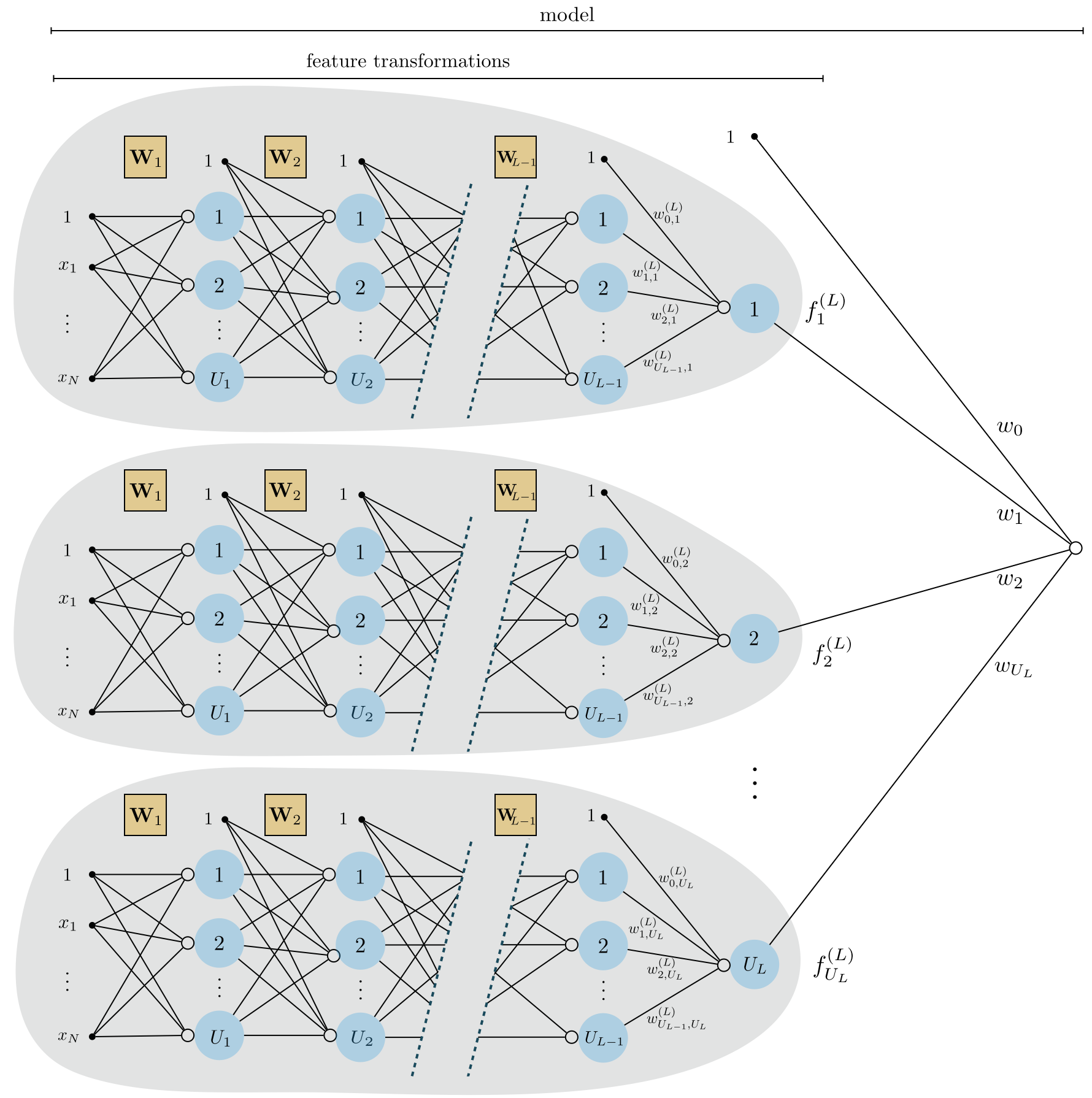
In general we will want to compute $B = U_L$ such $L$ layer units - a number we define - as feature transformations in supervised / unsupervised learning model
as we described in the previous Chapter where we introduced the idea of nonlinear learning. The $j^{th}$ of which looks like
\begin{equation} f^{\left(L\right)}_j\left(\mathbf{x}\right)=a\left(w^{\left(L\right)}_{0.j}+\underset{i=1}{\overset{U_{L-1}}{\sum}}{w^{\left(L\right)}_{i,j}}\,f^{(L-1)}_i\left(\mathbf{x}\right)\right) \end{equation}These are our feature transformations, which we implement in a feature_transforms module (as done repeatedly in Chapter 12) as follows.
Figure 8 shows a graphical representation of these feature transformations along with their linear combination - an $L$-layer neural network model whose algebraic form is given in (26).
Pythonic implementation of $L$ layer units¶To construct an effecient feature_transforms function we follow precisely the same steps we used in developing the single and two layer versions above. First note that our $L-1$ layer units can be expressed (using the notation introduced in the previous two Subsection) compactly as a generalization of equation (20)
We then construct a weight matrix $\mathbf{W}_L$ to contain all of the internal weights of our $L^{th}$ layer units by stacking our $j^{th}$ unit's weights into the $j^{th}$ column as
\begin{equation} \mathbf{W}_{L}=\left[\begin{array}{cccc} w_{0,1}^{\left(L\right)} & w_{0,2}^{\left(L\right)} & \cdots & w_{0,U_{L}}^{\left(L\right)}\\ w_{1,1}^{\left(L\right)} & w_{1,2}^{\left(L\right)} & \cdots & w_{1,U_{L}}^{\left(L\right)}\\ \vdots & \vdots & \ddots & \vdots\\ w_{U_{L-1},1}^{\left(L\right)} & w_{U_{L-1},2}^{\left(L\right)} & \cdots & w_{U_{L-1},U_{L}}^{\left(L\right)} \end{array}\right] \end{equation}Note that this matrix has dimensions $\left(U_{L-1} +1 \right)\times U_L$. With this compact matrix notation we can then express all $U_L$ of our $L$ layer units simulataneously in a single recursive vector-matrix computation
If we unwravel our notation our $L$ units can also be written as
\begin{equation} \mathbf{f}^{(L)} = \mathbf{a}\left(\mathbf{W}_{L}^T\mathring{\mathbf{a}}\left(\mathbf{W}_{L-1}^T\,\mathring{\mathbf{a}}\left( \cdots \mathbf{W}_{1}^T\mathring{\mathbf{x}}\right) \right)\right)\cdots ). \end{equation}In either case, we do indeed have that the $j^{th}$ element of this computation is our $j^{th}$ second layer unit
\begin{equation} \mathbf{f}^{(L)}_j = f^{\left(L\right)}_j\left(\mathbf{x}\right). \end{equation}Now we can construct our entire set of $U_L$ $L$ layer perceptron units very efficiently as a feature_transforms function that takes in x which we will call a - our input data - and the correctly sized matrices $\mathbf{W}_1$ through $\mathbf{W}_L$ for each layer of our perceptron. This will result in a long list of matrices
w = [W_1,W_2,W_3,...,W_L]
also known as a tensor.
In any case, below we provide an implementation based on the notation above for computing all of our $U_L$ second layer units effectively. Notice how this is precisely the code block we wrote for the two layer case above, only now we loop over $L$ weight matrices instead of just two.
# a feature_transforms function for computing
# U_L L layer perceptron units efficiently
def feature_transforms(a, w):
    # loop through each layer matrix
    for W in w:
        # pad with ones (to compactly take care of bias) for
        # current layer computation
        o = np.ones((1,np.shape(a)[1]))
        a = np.vstack((o,a))

        # compute linear combination of current layer units
        v = np.dot(a.T, W).T

        # pass through activation
        a = activation(v)
    return a
Before we look at a few examples, note that we can express our model using the sort of compact notation we employed in writing our set of two layer units so effectively. Using a notation to denote the weights of the linear combination as
and extend our vector $\mathbf{f}^{(L)}$ by tacking a $1$ on top of it - which as usual we denote by adding a $\mathring{}$ symbol to the top of notation as $\mathring{\mathbf{{f}}}^{(L)}$ - we can then write out the model in equation (16) quite compactly as
\begin{equation} \text{model}\left(\mathbf{x},\mathbf{w}\right) = \mathbf{w}_{L+1}^T\mathring{\mathbf{{f}}}^{(L)} \end{equation}where we use the notation $\mathbf{w}$ on the left hand side to denote all of the weights on the right - i.e., $\mathbf{w}_{L+1}$ and all weight matrices $\mathbf{W}_1$ through $\mathbf{W}_L$.
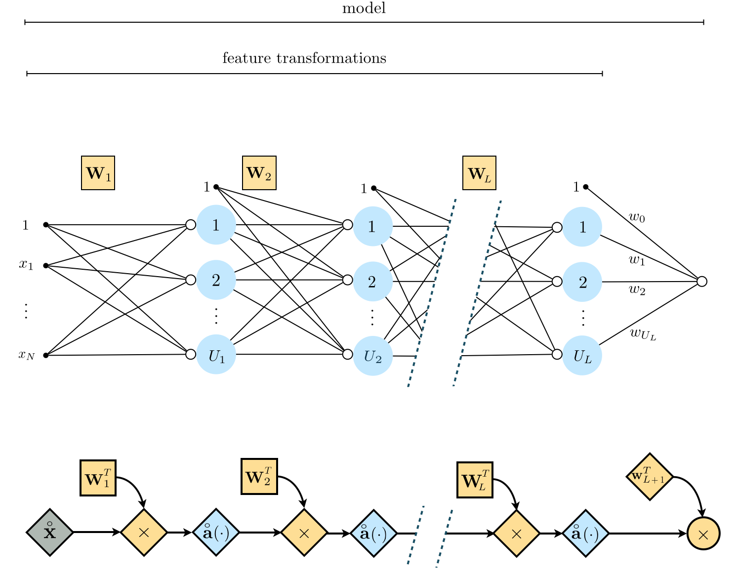
In Figure 9 we show a graphical representation of an $L$-layer network (top panel) along with its computational graph (bottom panel) employing once again our condensed notation described above.
Below we also provide a Python function initialize_network_weights that creates initial weights for a feedforward network, and also provides a simple interface for generating feedforward architectures with arbitrary numbers of layers. To create a desired network you simply input a comma-separated list called layer_sizes into the function of the following form
The initializer will then automatically create initial weight matrices (of the proper dimensions) $\mathbf{W}_1$ through $\mathbf{W}_L$ as well as the final weights for the linear combination in the prediction $\mathbf{w}$. We will see explicit examples using this functionality - as well as the previous Python functions - in the examples below.
# create initial weights for arbitrary feedforward network
def initialize_network_weights(layer_sizes, scale):
    # container for entire weight tensor
    weights = []

    # loop over desired layer sizes and create appropriately sized initial
    # weight matrix for each layer
    for k in range(len(layer_sizes)-1):
        # get layer sizes for current weight matrix
        U_k = layer_sizes[k]
        U_k_plus_1 = layer_sizes[k+1]

        # make weight matrix
        weight = scale*np.random.randn(U_k+1,U_k_plus_1)
        weights.append(weight)

    # re-express weights so that w_init[0] = omega_inner contains all
    # internal weight matrices, and w_init = w contains weights of
    # final linear combination in predict function
    w_init = [weights[:-1],weights[-1]]

    return w_init
In Section 12.3 we introduced the general nonlinear autoencoder, which consists of two (in general) nonlinear functions - an encoder $f_{\text{e}}$ and decoder $f_{\text{d}}$ - whose parameters we tune so that (ideally) the composition $f_{\text{d}}\left(\,f_{\text{e}}\left(\mathbf{x}\right)\right)$ forms the best nonlinear manifold on which the input data sits. That is, given a set of input points $\left\{\mathbf{x}_p\right\}_{p=1}^P$ we aim tune the parameters of our encoder / decoder pair so that ideally
for all of the datapoints. Just as with a supervised learner we can use a multilayer perceptron here - and for both encoding and decoding functions - which in combination provides us with an enormous amount of flexibility in terms of the sort of nonlinear manifolds we can uncover.
Below we plot out 9 random instances of an antoencoder function $f_{\text{d}}\left(\,f_{\text{e}}\left(\mathbf{x}\right)\right)$ where we have used a 5 hidden layer multilayer perceptron with 10 units in each layer for both functions, and the function sinc as an activation. In other words, below is plotted 9 instances of the function $f_{\text{d}}\left(\,f_{\text{e}}\left(\mathbf{x}\right)\right)$ where both $f_{\text{d}}$ and $f_{\text{e}}$ are 5 layer networks with randomly chosen weights in each instance. Each of examples shows the kind of nonlinear manifold we could potentially discover using such encoding/decoding functions.

In this example we demonstrate the usage of the Python functionality below to create an arbitrary feedforward network architecture to perform nonlinear regression using the toy dataset below.

Here we will use a 3 layer network with 10 units in each layer (we chose the number of units in each layer arbitrarily here). This will certainly overfit the dataset if we tune the parameters well!
In the next Python cell we create the handle list layer_sizes for our network and generate the initial weights.
# An example 4 hidden layer network, with 10 units in each layer
N = 1  # dimension of input
M = 1  # dimension of output
U_1 = 10; U_2 = 10; U_3 = 10; U_4 = 10;  # number of units per hidden layer

# the list defines our network architecture
layer_sizes = [N, U_1,U_2,U_3,U_4,M]

# generate initial weights for our network
w = initialize_network_weights(layer_sizes, scale = 0.5)
With all of our weights initialized we can then use gradient descent to tune them properly (here we used the normalized version). Below we define our least_squares cost function and run normalized gradient descent for 5000 iterations using a fixed steplength parameter $\alpha = 10^{-1}$. We can then examine the cost function history to make sure gradient descent is converging properly.

The cost function plot looks good! Taking the final weight from our history we can then evaluate testing points through our model function. In particular we can illustrate our nonlinear prediction - which we do below. We certainly do overfit, but this is not a surprise since our network is so flexible (and we optimized it quite well).

Here we use a network architecture to perform nonlinear classification using the following toy dataset. The dataset is shown 'from above' in the left panel, where red points belong to class $+1$ and blue points to class $-1$, and from the side in the right panel.

We will use the same network architecture used in the previous regression example here - 4 hidden layers with 10 units in each layer. Below we initialize the network, mirroring this step in the previous example.
# An example 4 hidden layer network, with 10 units in each layer
N = 2  # dimension of input
M = 1  # dimension of output
U_1 = 10; U_2 = 10; U_3 = 10;  # number of units per hidden layer

# the list defines our network architecture
layer_sizes = [N, U_1,U_2,U_3,M]

# generate initial weights for our network
w = initialize_network_weights(layer_sizes, scale = 0.5)
Now we can tune the weights of our network architecture using a softmax (or logistic) cost function. We provide a compact version of the softmax cost function below, and run normalized gradient descent for 5000 iterations using a steplength parameter $\alpha = 10^{-1}$.
With gradient descent run, we plot the cost function history at each step of gradient descent.

Finally, we visualize the fit provided by the final weights learned via gradient descent. Here it is harder to visually determine whether or not we have overfit when viewing the fit from above (in the left panel), since points from the two classes are so nicely separable by closed curves. However when you look at the fit from the side (in the right panel) you can see how the learned surface is extremely ripply (a sign that we overkilled this particular dataset using such a flexible network).

In this example we illustrate the use of multilayer perceptrons for both the encoder $f_{\text{e}}$ and decoder $f_{\text{d}}$ a general autoencoder function (see e.g., Section 12.3 for an introduction to the nonlinear autoencoder). Here for both functions we will use a 3 layer multilayer perceptron with 10 units in each layer and the tanh activation. We will then tune the parameters of both functions by minimizing the autoencoder cost function to uncover the proper nonlinear manifold on which the following dataset sits.

Below we initialize two multilayer perceptrons - one for each of the encoding and ecoding function.
### initialize encoder network ###
N = 2  # dimension of input
M = 1  # dimension of output
U_1 = 10; U_2 = 10; U_3 = 10;  # number of units per hidden layer

# the list defines our network architecture
layer_sizes = [N, U_1,U_2,U_3,M]

# generate initial weights for our network
w_encoder = initialize_network_weights(layer_sizes, scale = 0.5)

### initialize decoder network ###
N = 1  # dimension of input
M = 2  # dimension of output

# the list defines our network architecture
layer_sizes = [N, U_1,U_2,U_3,M]

# generate initial weights for our network
w_decoder = initialize_network_weights(layer_sizes, scale = 0.5)

# gather initializations for both encoder and encoder, package into single list
w = [w_encoder,w_decoder]
With our encoder and decoder constructed and initialized, we then minimize the corresponding autoencoder cost function over the dataset.

Having minimized the cost function appropriately we can now visualize the learned manifold (middle panel below) and the decoded version of the original dataset (right panel below) - i.e., the original dataset projected onto our learned manifold. We can also visualize how all of the data in this space is projected onto the learned manifold via a vector field plot, which we do in the bottom panel.


[1] W. S. McCulloch and W. Pitts. A logical calculus of the ideas immanent in nervous activity. The bulletin of mathematical biophysics, 5(4):115–133, 1943.
[2] D. O. Hebb. The organization of behavior: a neuropsychological theory. John Wiley & Sons, New York, 1949.
[3] F. Rosenblatt. The perceptron - a perceiving and recognizing automaton. Cornell Aeronautical Laboratory, 1957.