A common problem negatively affecting gradient descent in practice is when it is applied to minimize cost functions whose minima lie in a long narrow valley. We illustrate such a cost function in the right panel of Figure 1: a two-dimensional quadratic with elongated elliptic contours. A regular gradient descent step in this case (shown in solid red) does little to reduce the cost function evaluation because the negative gradient at $\mathbf{w}^{k}$, being perpendicular to the contour line at that point, points far away from the optimal direction (shown in dashed black) connecting $\mathbf{w}^{k}$ to the desired minimum located in the center.

Figure 1: From left to right, as the contours of a two-dimensional quadratic get more elongated, the gradient descent direction (red) diverges from the optimal direction (dashed black) connecting $\mathbf{w}^{k}$ to the desired minimum located in the center.

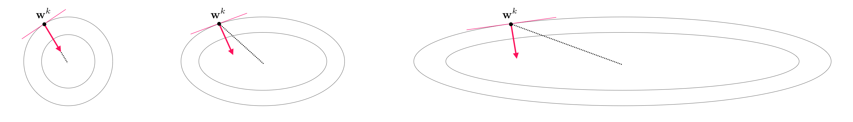
The progress of gradient descent is significantly slowed down due to the geometry of narrow valleys which causes gradient descent steps to zig-zag towards a solution. This problem motivates the concept of an old and simple heuristic known as the momentum term, added to the standard gradient descent. The momentum term is a simple weighted difference of the subsequent $k^{th}$ and $(k−1)^{th}$ gradient steps, i.e., $\beta \left(\mathbf{w}^k - \mathbf{w}^{k-1}\right)$ for some $\beta >0$. As illustrated in Figure 2, the momentum term is designed to even out the zig-zagging effect of regular gradient descent by tilting back the gradient steps (that move perpendicular to the contours of the cost function) towards the center where the minimum lies. The $k^{th}$ gradient descent step as well as the $k^{th}$ gradient descent step with momentum are shown in Figure 2, colored red and blue respectively.

Figure 2: A figurative illustration of a gradient descent (red) and a momentum-adjusted gradient descent (blue) step toward the minimum of a function located at the center of a long narrow valley. The addition of the momentum term (dashed black arrow) pushes the negative gradient toward the function's minimum, thus ameliorating the zig-zagging inherent in standard gradient descent.

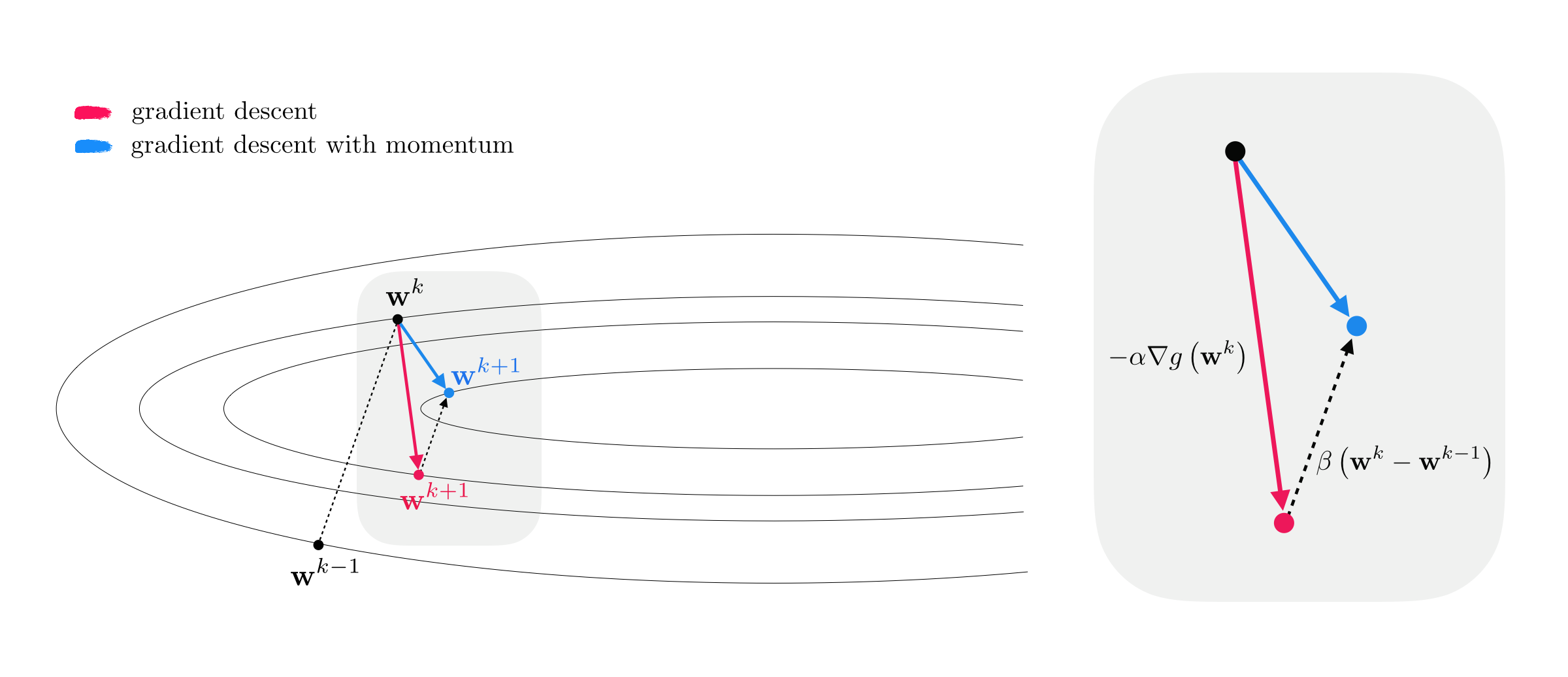
To derive the momentum-adjusted gradient step update we add the momentum term $\beta \left(\mathbf{w}^k - \mathbf{w}^{k-1}\right)$ to the standard gradient descent update at $\mathbf{w}^k$, giving

\begin{equation} \mathbf{w}^{k+1} = \mathbf{w}^k - \alpha \nabla g\left(\mathbf{w}^k\right) + \beta \left(\mathbf{w}^{k} - \mathbf{w}^{k-1}\right) \end{equation}

where the parameter $0< \beta < 1$ trades off the direction from the negative gradient and momentum term. If desired, $\beta$ can be adjusted as well at each iteration. When tuned properly the adjusted gradient descent step with momentum is known empirically to significantly improve the convergence of gradient descent (see e.g., [1]).

The momentum update in equation (1) is often written in an equivalent manner by subtracting $\mathbf{w}_k$ from both sides of equation (1), and dividing both sides by $-\alpha$ to get

\begin{equation} \frac{1}{-\alpha}\left(\mathbf{w}^{k+1}-\mathbf{w}^k\right) = \nabla g\left(\mathbf{w}^k\right) - \frac{\beta}{\alpha} \left(\mathbf{w}^{k} - \mathbf{w}^{k-1}\right) \end{equation}

Denoting the left hand side of (2) by a new variable $\mathbf{z}^{k+1} = \frac{1}{-\alpha}\left(\mathbf{w}^{k+1}-\mathbf{w}^k\right) $, we can rewrite it as

\begin{equation} \mathbf{z}^{k+1} = \nabla g\left(\mathbf{w}^k\right) +\beta\, \mathbf{z}^{k} \end{equation}

Equation (3) together with a simple rearrangement of $\mathbf{z}^{k+1} = \frac{1}{-\alpha}\left(\mathbf{w}^{k+1}-\mathbf{w}^k\right)$ give the following momentum update, done in two de-coupled steps

\begin{equation} \begin{array} \ \mathbf{z}^{k+1} = \beta\,\mathbf{z}^{k} + \nabla g\left(\mathbf{w}^k\right) \\ \mathbf{w}^{k+1} = \mathbf{w}^{k} - \alpha \, \mathbf{z}^{k+1} \end{array} \end{equation}

which is equivalent to the original derivation in equation (1).

In the Python cell below we modify our gradient descent code by adding beta as an input parameter, and adjusting the gradient descent step as derived in equation (4).

def gradient_descent(g,w,alpha,max_its,beta,version):    
    # flatten the input function, create gradient based on flat function
    g_flat, unflatten, w = flatten_func(g, w)
    grad = compute_grad(g_flat)

    # record history
    w_hist = []
    w_hist.append(unflatten(w))

    # start gradient descent loop
    z = np.zeros((np.shape(w)))      # momentum term
    
    # over the line
    for k in range(max_its):   
        # plug in value into func and derivative
        grad_eval = grad(w)
        grad_eval.shape = np.shape(w)

        ### normalized or unnormalized descent step? ###
        if version == 'normalized':
            grad_norm = np.linalg.norm(grad_eval)
            if grad_norm == 0:
                grad_norm += 10**-6*np.sign(2*np.random.rand(1) - 1)
            grad_eval /= grad_norm
            
        # take descent step with momentum
        z = beta*z + grad_eval
        w = w - alpha*z

        # record weight update
        w_hist.append(unflatten(w))

    return w_hist

Example 1. Using momentum to speed up the minimization of simple quadratic functions

A simple quadratic cost function in 2-d takes the form

\begin{equation} g(\mathbf{w}) = a + \mathbf{b}^T\mathbf{w} + \mathbf{w}^T\mathbf{C}\mathbf{w} \end{equation}

where $a$ is a scalar, $\mathbf{b}$ a $2\times1$ vector, and $\mathbf{C}$ a $2\times2$ matrix.

Setting $a = 0$, $\mathbf{b} = \begin{bmatrix} 0 \\ 0 \end{bmatrix}$, and $\mathbf{C} = \begin{bmatrix} 1\,\,0 \\ 0 \,\, 12\end{bmatrix}$ in the Python cell below we run gradient descent with ($\beta = 0.3$) and without ($\beta = 0$) momentum for a maximum of $10$ iterations with the steplength parameter set to $\alpha = 0.08$ in both cases.

As can be seen the addition of the momentum term (bottom panel) corrects the zig-zagging effect of standard gradient, achieving a lower solution with the same number of iterations.

As illustrated in Figure 1, the longer and narrower the valley where the minimum lies in, the more severe the zig-zagging effect becomes, and the larger we should set $\beta$ as a result.

We repeat the previous experiment this time using another quadratic function with $a = 0$, $\mathbf{b} = \begin{bmatrix} 2 \\ 0 \end{bmatrix}$, and $\mathbf{C} = \begin{bmatrix} 0\,\,0 \\ 0 \,\, 12\end{bmatrix}$. We run gradient descent with ($\beta = 0.7$) and without ($\beta = 0$) momentum for a maximum of $20$ iterations with the steplength parameter set to $\alpha = 0.08$ in both cases.

Example 2. Using momentum to speed up the minimization of linear two-class classification

The use of momentum is not limited to convex costs as non-convex functions can too have problematic long narrow valleys. In this example we compare the quality of solutions achieved by standard gradient descent and its momentum-adjusted version using the (non-convex) logistic Least Squares cost function on a simulated 1-d classification dataset. Both algorithms are initialized at the same point, and run for $25$ iterations with $\alpha = 1$.

Moving the slider widget from left to right animates the optimization path taken by each algorithm as well as the corresponding fit to the data with (blue) and without (magenta) momentum.

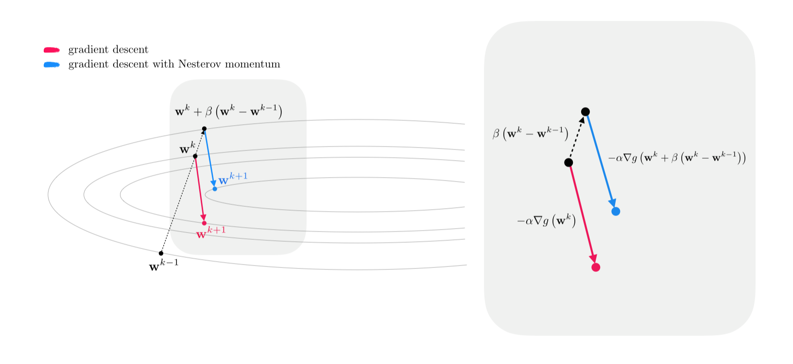
Another popular variant of the momentum method is derived when a momentum term, i.e., $\beta\left(\mathbf{w}^k-\mathbf{w}^{k-1}\right)$, is added not only to the gradient descent update as in Equation (1) but also to the inside of the gradient term itself, giving

\begin{equation} \mathbf{w}^{k+1} = \mathbf{w}^k - \alpha \nabla g\left(\mathbf{w}^k+\beta\left(\mathbf{w}^k-\mathbf{w}^{k-1}\right)\right) + \beta \left(\mathbf{w}^{k} - \mathbf{w}^{k-1}\right) \end{equation}

Denoting $\mathbf{w}^k+\beta\left(\mathbf{w}^k-\mathbf{w}^{k-1}\right)$ as $\mathbf{\tilde w}^k$, the momentum step in (6), typically referred to as the Nesterov momentum, can be thought of and written as a regular gradient descent step at $\mathbf{\tilde w}^k$

\begin{equation} \mathbf{w}^{k+1} = \mathbf{\tilde w}^k - \alpha \nabla g\left(\mathbf{\tilde w}^k\right) \end{equation}

In Figure 3, through a figurative illustration, we show how taking a gradient step at $\mathbf{\tilde w}^k$ (instead of $\mathbf{w}^k$) helps ameliorate the zig-zagging phenomenon associated with long, narrow valleys.

Figure 3: A figurative illustration of a gradient descent (red) and a Nesterov momentum-adjusted gradient descent (blue) step toward the minimum of a function located at the center of a long narrow valley.

The Nesterov momentum update in (6) is sometimes written in two steps, equivalently as

\begin{equation} \begin{array} \ \mathbf{z}^{k+1} = \beta\,\mathbf{z}^{k} + \nabla g\left(\mathbf{w}^k-\alpha\beta\,\mathbf{z}^{k}\right) \\ \mathbf{w}^{k+1} = \mathbf{w}^{k} - \alpha \, \mathbf{z}^{k+1} \end{array} \end{equation}

Practically speaking both momentum updates in (1) and (6) are similarly effective.

Example 3. Using momentum for optimizing a multi-layer perceptron

In this Example we use gradient descent with and without momentum on a two-class classification dataset collected for the task of face detection, consisting of $P=10,000$ face and non-face images.

Once the data is loaded, we move on to initiate a supervised learning instance using our deep learning library, create a four-layer neural network basis consisting of $10$ units in each layer, and choose an activation function (here, ReLU), data normalization scheme (here, standard normalization) as well as the cost function (here, softmax).

We now run gradient descent twice for $200$ iterations using the same initialization and steplength parameter, once without momentum ($\beta=0$) and once with momentum parameter set to $\beta=0.9$.

References

[1] Ning Qian. On the momentum term in gradient descent learning algorithms. Neural Networks, 12(1) 145–151, 1999.