code

share


To perform supervised or unsupervised tasks on image data, like object detection or image compression (dimension reduction) one could always use the (raw) pixel values directly as features. This naive approach however has been shown experimentally to produce low quality results in virtually all machine learning tasks involving natural images*. An alternative, more efficient approach would be to represent an image by making use of its edge content, as illustrated in Figure 1 which shows an image (left panel) along with a corresponding image comprised of its most prominent edges (right panel).
The edge-detected image in the right panel of Figure 1 is an efficient representation of the original image in the left panel in the sense that we can still tell what the image contains while throwing away a lot of information from the majority of the pixels that do not belong to any edges.
This is true in general: the distinguishing information in a natural image is largely contained in the relatively small number of edges in an image [1,2]. Interestingly, this fact is also confirmed by visual studies performed largely on frogs, cats, and primates, where a subject is shown visual stimuli while electrical impulses are recorded in a small area in the subject's brain where visual information is processed. These studies have determined that individual neurons involved in early stages of visual processing roughly operate by identifying edges [3,4]. Each neuron therefore acts as a small "edge detector," locating edges in an image of a specific orientation and thickness, as shown in Figure 2. It is thought that by combining and processing these edge detected images, humans and other mammals "see."
Motivated by our discussion in the previous subsection, here we design a feature extraction scheme based on the information provided by edges of different orientation within an image. This is indeed the basis of many popular engineered features, including Histogram of Oriented Gradients (HoG) [5] and Scale-Invariant Feature Transform (SIFT) [6].
Edges can be detected within an image using convolution. Recall from our post on convolution operation, that convolving an image with appropriate horizontal and vertical kernels gives image gradients in those directions where large pixel values indicate high edge content. Additional kernels can be added to the mix to detect edges that are not horizontal /vertical but are at an incline. For example, the eight kernels shown below each correspond to one of eight equally (angularly) spaced edge orientations, starting from 0 degrees with seven additional orientations at increments of 45 degrees.

To capture the total 'edge content' of an image in each direction, we convolve it with the appropriate kernel, pass the results through a rectified linear unit (ReLU) to remove negative entries, and sum up the remaining positive pixel values. Denoting the input image by $x$ and the convolution kernels by $w_1,\,\ldots,\,w_8$, this gives us eight features $f_1,\,\ldots,\,f_8$ to represent $x$, defined as
\begin{equation} f_{i}=\underset{\text{all pixels}}{\sum}\text{max}\left(0,\,w_{i}*x\right) \qquad i=1,\,\ldots,\,8 \end{equation}We use ReLU in (1) so that large positive values in $w_{i}*x$ do not get canceled out by possible large negative values in it. Notice, we are not discarding any information by removing negative entries in $w_{i}*x$. In fact it can be easily verified that those negative entries are identical to the positive entries in $w_{j}*x$, where $w_i$ and $w_j$ are kernels associated to opposing directions.
Stacking all $f_i$'s together into a single vector $\mathbf{f}$ we now have a feature representation for $x$ in the form of an edge histogram which is typically normalized to have unit length (in the $\ell_2$ or $\ell_1$ sense). In the Python cell below we plot an input image (in this case a circle), along with the convolution plots of the input image with each of the eight kernels in Figure 3 (after passing through ReLU), and the final histogram representation of the image in the last column.

The feature extractor we have designed so far may work well in overly simplistic scenarios, e.g. distinguishing a circle from a triangle or a square. But even then it fails to distinguish between a circle and a star, as their feature representations end up to be identical due to the symmetry of both shapes.

Real images used in practice are significantly more complicated than these simplistic geometrical shapes and summarizing them using just eight features would be extremely ineffective. To fix this issue, instead of computing the edge histogram features over the entire image as done in (1), we break the image into relatively small patches (that may be overlapping), compute features for each patch
\begin{equation} f_{i,\,j}=\underset{j\,\text{th patch}}{\sum}\text{max}\left(0,\,w_{i}*x\right) \qquad i=1,\,\ldots,\,8 \end{equation}and then concatenate the results to arrive at the final feature representation. This process, i.e., breaking the image into small patches and representing each patch via the sum of its pixels, is referred to as pooling (or more accurately sum-pooling) in the parlance of machine learning and computer vision, and is shown pictorially in Figure 4 for an example matrix.
Procedurally, the pooling operation is similar to convolution with only two differences. First, with pooling the sliding window can jump multiple pixels at a time depending on how much overlap is required between adjacent windows/patches. The number of pixels the sliding window is shifted is typically referred to as the stride. Notice, with convolution the stride is always 1.
The second difference between convolution and pooling is how the content of the sliding window is processed and then summarized as a single value in each case. Recall that with convolution, the input function to the sliding_window module computes the sum of the entry-wise product between the window and a kernel. With pooling on the other hand, there is no kernel and we simply sum up all the pixels inside the kernel.
Slightly modifying the sliding_window module from our post on convolution operation to include stride as an input parameter, we have
def sliding_window(image, window_size, func, stride):

    # grab image size, set container for results
    image_size = np.shape(image)[0]
    results = []

    # slide window over input image
    for i in np.arange(0, image_size - window_size + 1, stride):
        for j in np.arange(0, image_size - window_size + 1, stride):
            # extract window from the image
            window = image[i:i+window_size,j:j+window_size]

            # process using the input 'func' (here the convolution function)
            processed_window = func(window)

            # store the results
            results.append(processed_window)

    # return results in numpy array format
    return np.array(results)
Finally to pool an image one can call sliding_window with
pool_function = lambda window: np.sum(window)
as the input function.
Putting together all the components discussed in the previous subsection, i.e., convolution, ReLU, and pooling, we show the end-to-end image feature extraction pipeline in Figure 5.
The module make_feature_map below takes in a single image and a single kernel, computes their convolution, and pool the result after passing through a ReLU module.
def make_feature_map(image, kernel):

    # parameters for transform
    kernel_size = kernels[0].shape[0]
    pool_kernel_size = 3
    stride = 2

    # pad image with zeros
    padded_image = self.pad_image(image,kernel_size)

    # window image
    feature_map = self.sliding_window_image(padded_image,kernel_size,stride = 1,func = self.conv_function)

    # reshape convolution feature map into array
    feature_map = np.reshape(feature_map,(np.shape(image)))

    # now shove result through nonlinear activation
    feature_map = self.activation(feature_map)

    #### now pool / downsample feature map, first window then pool on each window
    max_pool = self.sliding_window_image(feature_map,pool_kernel_size,stride = stride,func = self.pool_function)

    # reshape into new tensor
    max_pool = np.reshape(max_pool, (int((np.size(max_pool))**(0.5)),int((np.size(max_pool))**(0.5))))

    return max_pool
Notice how we used the same module sliding_window to perform both convolution and pooling, albeit with different stride and processing function.
To extract the full feature representation of entire image dataset we can use make_feature_map and construct one feature map at a time by looping through all images, and for each image constructing a feature map for each convolution kernel (again by explicitly looping through the kernels). This is implemented in the conv_layer module below.
 # main convolution layer definition
def conv_layer(self,images,kernels):
    #### create image tensor from input images
    image_tensor = np.reshape(images,(np.shape(images)[0],int((np.shape(images)[1])**(0.5)),int( (np.shape(images)[1])**(0.5))),order = 'F')

    #### loop over each image, shove through filters and make feature maps, then downsample and pool
    new_tensors = []

    #### loop over images
    for image in image_tensor:
        #### loop over kernels and construct feature map for each kernel
        downsampled_feature_maps = []
        for kernel in kernels:
            self.kernel = kernel
            downsampled_map = self.make_feature_map(image,kernel)
            downsampled_feature_maps.append(downsampled_map)

        ## re-shape downsampled_feature_maps and store
        new_tensors.append(downsampled_feature_maps)

    # reshape new tensor properly
    new_tensors = np.array(new_tensors)
    new_tensors = np.reshape(new_tensors, (np.shape(new_tensors)[0],np.shape(new_tensors)[1],np.shape(new_tensors)[2]*np.shape(new_tensors)[3]))
    new_tensors = np.reshape(new_tensors, (np.shape(new_tensors)[0],np.shape(new_tensors)[1]*np.shape(new_tensors)[2]),order = 'F')

    return new_tensors
Putting all pieces together into a python class we now have a simple convnet module wherein the feature maps are calculated one at a time, using a host of nested for-loops. This means computation will be quite slow. However, this can still be used in theory as a fixed convolutional feature extractor or as a convolutional layer in a convnet.
While the con_layer coded up in the previous subsection works accurately, in practice its Pyhton implemetation is extremely inefficient, particularly for meduim- to large-sized datasets, due to the nested for-loops involved!
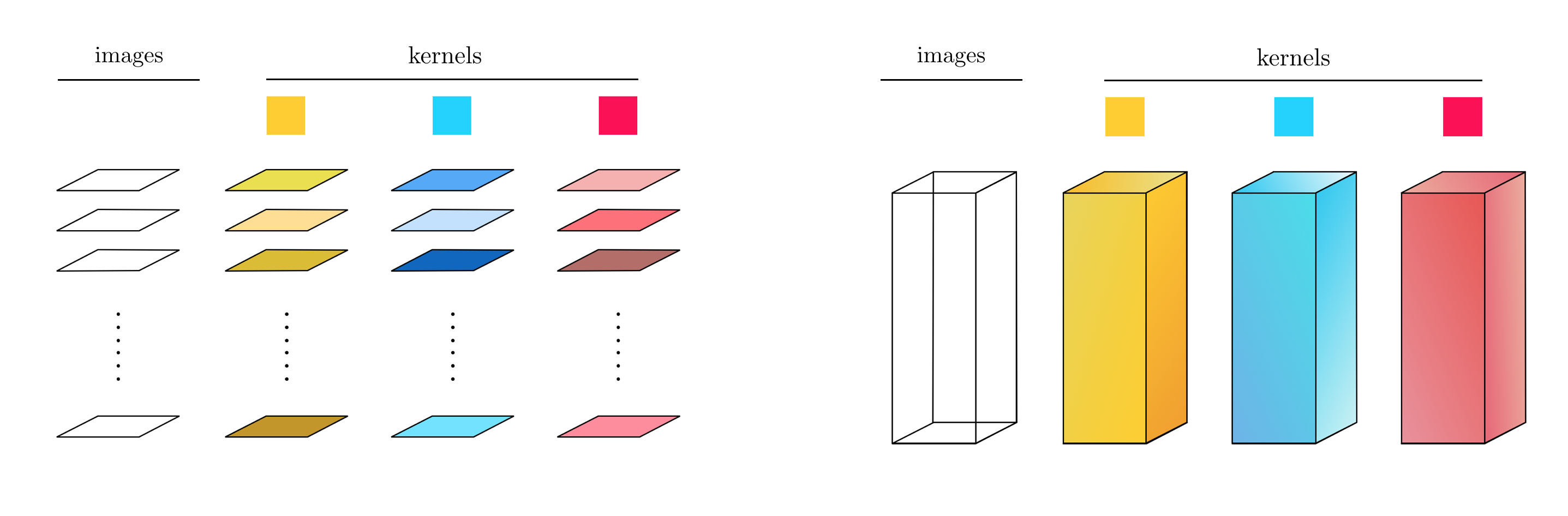
By carefully thinking about how convolutional feature maps are constructed on a set of images we can re-write the conv_layer in a much more efficient manner by employing tensors - i.e., three (and higher) dimensional matrices. The idea here, as shown pictorially in the right panel of Figure 7, is to process the entire stack (tensor) of images simultaneously, thereby minimizing the number of explicit for-loops required.
class tensor_conv_layer:
    # convolution function
    def conv_function(self,tensor_window):
        tensor_window = np.reshape(tensor_window,(np.shape(tensor_window)[0],np.shape(tensor_window)[1]*np.shape(tensor_window)[2]))
        t = np.dot(self.kernels,tensor_window.T)
        return t

    # pooling / downsampling parameters
    def pool_function(self,tensor_window):
        t = np.max(tensor_window,axis = (1,2))
        return t

    # activation
    def activation(self,tensor_window):
        return np.maximum(0,tensor_window)

    # pad image with appropriate number of zeros for convolution
    def pad_tensor(self,tensor,kernel_size):
        odd_nums = np.array([int(2*n + 1) for n in range(100)])
        pad_val = np.argwhere(odd_nums == kernel_size)[0][0]
        tensor_padded = np.zeros((np.shape(tensor)[0], np.shape(tensor)[1] + 2*pad_val,np.shape(tensor)[2] + 2*pad_val))
        tensor_padded[:,pad_val:-pad_val,pad_val:-pad_val] = tensor
        return tensor_padded

    # sliding window for image augmentation
    def sliding_window_tensor(self,tensor,window_size,stride,func):
        # grab image size, set container for results
        image_size = np.shape(tensor)[1]
        results = []

        # slide window over input image with given window size / stride and function
        for i in np.arange(0, image_size - window_size + 1, stride):
            for j in np.arange(0, image_size - window_size + 1, stride):
                # take a window of input tensor
                tensor_window =  tensor[:,i:i+window_size, j:j+window_size]

                # now process entire windowed tensor at once
                tensor_window = np.array(tensor_window)
                yo = func(tensor_window)

                # store weight
                results.append(yo)

        # re-shape properly
        results = np.array(results)
        results = results.swapaxes(0,1)
        if func == self.conv_function:
            results = results.swapaxes(1,2)
        return results

    # make feature map
    def make_feature_tensor(self,tensor):
        # create feature map via convolution --> returns flattened convolution calculations
        conv_stride = 1
        feature_tensor = self.sliding_window_tensor(tensor,self.kernel_size,conv_stride,self.conv_function)

        # re-shape convolution output ---> to square of same size as original input
        num_filters = np.shape(feature_tensor)[0]
        num_images = np.shape(feature_tensor)[1]
        square_dim = int((np.shape(feature_tensor)[2])**(0.5))
        feature_tensor = np.reshape(feature_tensor,(num_filters,num_images,square_dim,square_dim))

        # shove feature map through nonlinearity
        feature_tensor = self.activation(feature_tensor)

        # pool feature map --- i.e., downsample it
        pool_stride = 2
        pool_window_size = 3
        downsampled_feature_map = []
        for t in range(np.shape(feature_tensor)[0]):
            temp_tens = feature_tensor[t,:,:,:]
            d = self.sliding_window_tensor(temp_tens,pool_window_size,pool_stride,self.pool_function)
            downsampled_feature_map.append(d)
        downsampled_feature_map = np.array(downsampled_feature_map)

        # return downsampled feature map --> flattened
        return downsampled_feature_map

    # our normalization function
    def normalize(self,data,data_mean,data_std):
        normalized_data = (data - data_mean)/(data_std + 10**(-5))
        return normalized_data

    # convolution layer
    def conv_layer(self,tensor,kernels):
        #### prep input tensor #####
        # pluck out dimensions for image-tensor reshape
        num_images = np.shape(tensor)[0]
        num_kernels = np.shape(kernels)[0]

        # create tensor out of input images (assumed to be stacked vertically as columns)
        tensor = np.reshape(tensor,(np.shape(tensor)[0],int((np.shape(tensor)[1])**(0.5)),int( (np.shape(tensor)[1])**(0.5))),order = 'F')

        # pad tensor
        kernel = kernels[0]
        self.kernel_size = np.shape(kernel)[0]
        padded_tensor = self.pad_tensor(tensor,self.kernel_size)

        #### prep kernels - reshape into array for more effecient computation ####
        self.kernels = np.reshape(kernels,(np.shape(kernels)[0],np.shape(kernels)[1]*np.shape(kernels)[2]))

        #### compute convolution feature maps / downsample via pooling one map at a time over entire tensor #####
        # compute feature map for current image using current convolution kernel
        feature_tensor = self.make_feature_tensor(padded_tensor)

        feature_tensor = feature_tensor.swapaxes(0,1)
        feature_tensor = np.reshape(feature_tensor, (np.shape(feature_tensor)[0],np.shape(feature_tensor)[1]*np.shape(feature_tensor)[2]),order = 'F')

        return feature_tensor
In this Example we compare the speeds of our naive versus tensor-based convolution layer implementations using the set of eight edge detecting kernels shown previously in Section 14.2.2.
To give a sense of just how much edge-based features improve our ability to detect visual objects we now perform a simple experiment on a subset of the the MNIST training dataset, consisting of $10,000$ $28 \times 28$ images of handwritten digits. A sample of MNIST images is shown below.

Now we create a set of fixed convolution features (using edge detecting kernels) - first using our naive implementation naive_conv_layer.
# start timer
startTime= time.time()

feature_maps_1 = naive_conv_test.conv_layer(x, kernels)

# finish timing
timeElapsed=time.time()-startTime

print('Time elpased in seconds:', timeElapsed)
And our more effecient tensor-based implementation tensor_conv_layer.
# start timer
startTime= time.time()

feature_maps_2 = tensor_conv_test.conv_layer(x, kernels)

# finish timing
timeElapsed=time.time()-startTime

print('Time elpased in seconds:', timeElapsed)
In general, the tensor-based implementation is two to three orders of magnitude faster.
Having shown in Example 1 how to compute edge-based features from the MNIST dataset efficiently, in this Example we use them to train a classifier to see whether using them as input to a multilayer perceptron provides an advantage over naive usage of raw pixel values as features. Note here we use the entire training portion of the MNIST dataset (consisting of $60,000$ points).
First, we classify the data using raw pixel values, employing a single hidden layer neural network with $10$ units, the maxout function as activation, and multiclass softmax cost function. Here we use $80\%$ of the data for training, and the remaining portion for validation. Below we plot the training and validation histories from this run, where we achieve around $94.8\%$ accuracy on the test set.

We now repeat this experiment this time using edge-based features extracted in Example 1 as input to our single hidden layer neural network. Here we use the same training / validation split of the data, and the same number of gradient descent steps. Overall we achieve a validation accuracy of around $96.5\%, a significant improvement.

Our feature extraction scheme shown in Figure 5 has several adjustable parameters/settings including:
These parameters, being all discrete in nature, are tuned by trail and error using cross-validation. One can easily show that the total number of edge-based features created using this pipeline, in terms of parameters given above, can be computed as
\begin{equation} k\, \left(\left\lfloor \frac{N_1 - r}{s}\right\rfloor +1\right)\left(\left\lfloor \frac{N_2 - r}{s}\right\rfloor +1\right) \end{equation}* A natural image is an image a human being would normally be exposed to like a forest or outdoor scene, cityscapes, other people, animals, the insides of buildings, etc.
[1] Horace Barlow. Redundancy reduction revisited. Network: Computation in Neural Systems, 12(3) 241–253, 2001.
[2] Horace Barlow. The coding of sensory messages. In Current Problems in Animal Behavior, pp. 331–360, 1961.
[3] Judson P Jones and Larry A Palmer. An evaluation of the two-dimensional gabor filter model of simple receptive fields in cat striate cortex. Journal of Neurophysiology, 58(6)1233–1258, 1987.
[4] Stjepan Marcelja. Mathematical description of the responses of simple cortical cells. JOSA, 70(11) 1297–1300, 1980.
[5] Navneet Dalal and Bill Triggs. Histograms of oriented gradients for human detection. In Computer Vision and Pattern Recognition, 2005. CVPR 2005. IEEE Computer Society Conference on, volume 1, pp. 886–893. IEEE, 2005.
[6] David G. Lowe. Distinctive image features from scale-invariant keypoints. International Journal of Computer Vision, 60(2) 91–110, 2004.
[7] Jianguo Zhang et al. Local features and kernels for classification of texture and object categories: A comprehensive study. International Journal of Computer Vision 73(2) 213–238, 2007.