code

share


In this Section we discuss a popular subspecies of fixed order dynamic systems - called recurrence relations. Instead of constructing an output sequence based on a given input sequence, these systems define input sequence themselves. Such systems are used throughout various science and engineering disciplines and go by many names, including recurrence relations (of course), difference equatinos, dynamical systems, and chaotic systems, and Markov Chains to name just a few.
With the general dynamic systems we saw in the previous Section we use a given input sequence $x_1,\,x_2,\,...,x_T$ to construct a new output sequence $h_1,\,h_2,...,h_T$. This output sequence is some filtered (e.g., smoothed) version of the original input, like the moving average. To construct such a sequence of general order $\mathcal{O}$ we set our initial conditions $h_1 = \gamma_1,\,h_2 = \gamma_2,...,h_\mathcal{O} = \gamma_{\mathcal{O}}$, and recurse on a generic update formulae
\begin{equation} h_{t} = f\left(x_{t-1},...,x_{t-\mathcal{O}}\right) \,\,\,\,\, \,\,\,\,\,\,\, t = \mathcal{O} + 1,...,T. \\ \end{equation}to construct the remaining entries.
A popular special instance of this kind of relationship, called a recurrence relation, simply defines an input sequence in terms of itself in the same sort of fashion as
\begin{equation} x_{t} = f\left(x_{t-1},...,x_{t-\mathcal{O}}\right) \,\,\,\,\, \,\,\,\,\,\,\, t = \mathcal{O} + 1,...,T. \\ \end{equation}In other words, we do not begin with an input sequence, instead we generate one by recursing on a set of formulae of the form above. We again have initial conditions to set, but these are simply the first $\mathcal{O}$ entries of the generated input sequence $x_1 = \gamma_1,\,x_2 = \gamma_2,...,x_\mathcal{O} = \gamma_{\mathcal{O}}$. Because they are used for modeling purposes in such a wide variety of fields, these sorts of fixed order dynamic systems go by many names including: recurrence relations, difference equations, dynamical systems, chaotic systems, to name a few.
Before diving into any more formal details, lets examine a few examples of such dynamic systems.
The simple recurrence relation of order $\mathcal{O} = 1$
generates a sequence that exhibits exponential growth. Here $\gamma$, $w_0$, and $w_1$ are constants which we can set to any values we please, and the function $f$ is (obviously) linear and given by $f\left(x\right) = w_0 + w_1x$. As with the generic dynamical system we saw in the previous Section, in generative cases like this one we still call the value assigned to $x_1 = \gamma$ as the initial condition. However unlike the generic dynamic system, in the generative case here the setting of this initial condition can significantly alter the trajectory of a sequence generated by such a system (as can the parameters of the update formula).
Below we show two example sequences of length $T = 10$. In the first, shown in the left panel below, we set the initial condition $x_1 = 2$ and $w_0 = 0$ and $w_1 = 2$. Note while each point in the sequence increases linearly from step to step, the data overall is increasing exponentially upwards. In the right panel we use an initial condition of $x_1 = 1$ with $w_0 = -2$ and $w_1 = 2$. This data - while decreasing linearly at each step - globally is decreasing exponentially.

You can see algebraically how the update step above leads to exponential behavior by 'rolling back' the formula to its initial condition at a given value of $t$. For example, say $w_0 = 0$ in the general exponential growth model above i.e., that our system takes the form
\begin{equation} \begin{array} \ x_1 = \gamma \\ x_{t} = w_1x_{t-1}. \end{array} \end{equation}Then if we roll back the update step - replacing $x_{t-1}$ with its update - we can write the update step above for $x_t$ as
\begin{equation} x_t = w_1x_{t-1} = w_1 \cdot w_1 x_{t-2} = w_1^2x_{t-2}. \end{equation}If we continue, subsituting in the update formula for $x_{t-2}$ and then likewise $x_{t-3}$ and so forth we can write the formula above equivalently as
\begin{equation} x_t = w_1^t \,x_{1}^{\,} \end{equation}which does indeed show how the sequence behaves exponentially depending on the coeffecient value $w_1$. Setting $w_0 \neq 0$ one can show a similar exponential relationship throughout the sequence by similarly rolling back to the initial condition.
This kind of dynamic system is precisely what we use when calculating compound interest on a loan. For example, the run shown in the left panel above (could be interpreted (if we suppose $p$ has a unit of weeks and $x_p$ dollars) as showing the total amount owed on a loan of $x_1 = \$2$ at an interest rate of $100\%$ ($w_1 = 2$) per week over the period of $10$ weeks. This kind of ridiculous high interest loan is often made by 'loansharks' in the movies, and by predatory 'payday loan' shops in the real world.
More generally the formula for compound interest (when none of the principal or interest is repaid at each period) on an initial loan of $x_1$ dollars is a version of the linear growth model above
\begin{equation} x_{t} = \left(1 + \text{interest rate}\right)x_{t-1}. \end{equation}In other words, it is the exponential growth model with $w_0 = 0$ and $w_1 = \left(1 + \text{interest rate}\right)$.
This sort of model is also used as a simple model for uncapped population growth. For example, suppose a single species of creature (bacteria, bunny rabbits, humans, whatever) live alone on a planet that has an infinite amount of space, resources, etc., Suppose at the start of the universe there are $2$ creatures, and after each period of time (e.g., a day) they reproduce at a rate of $100\%$. Since there are infinite resources in this universe they can go on reproducing forever, reproducing at an exponential rate. This scenario can also be interpreted as the example in the left panel above (where $x_1 = 2$ denotes the initial number of creatures and $w_1 = 2$ the growth rate).
Just like compound interest, the uncapped population growth model falls into the same kind of framework as we saw above as
\begin{equation} x_{t} = \left(\text{growth rate per period}\right)x_{t-1}. \end{equation}In other words, it is the exponential growth model with $w_0 = 0$ and $w_1 = \left(1 + \text{growth rate per period}\right)$.
One generalization of the exponential growth model in the previous Example is the so-called autoregressive system, whose steps each consist of a linear combination of $\mathcal{O}$ prior elements with the addition of some small amount of noise at each step. This general order $\mathcal{O}$ system takes the form
where $\epsilon_t$ denotes the small amount of noise introduced at each step. Sequences generated via this dynamic system tend to look like the sort of noisy financial time series commonly seen in practice after a centering procedure has been used to 'detrend' the data. We show two such examples below, each is a $\mathcal{O} = 4$ model whose initial conditions and weights are chosen at random, with standard normal noise used at each step.

In this example we illustrate several examples of input data generated via the classical logistic system, defined as follows
In other words, this is a dynamic system recurrence relation with update function $f\left(x\right) = wx\left(1 - x\right)$.
It is called a logistic system because (like logistic functions themselves) it arises in the modeling of population growth under the assumption that resources in an environment are limited. The modeling idea is basically this: if $x_p$ denotes the population of a single species of creature (e.g., bacterium, bunny rabbits, humans, whatever) in a closed system with a maximum amount of space / resources the growth rate of a population cannot follow the exponential rate detailed in the previous example forever. In the beginning, when there are not too many of the creatures, the growth can indeed be exponential - thus the first part of the equation above $wx_{p}$ (the exponential growth we saw previously). But at a certain point, when space and resources become limited, competition for survival causes the growth rate to slow down. Here this concept is modeled by the second portion of the equation above: $\left(1 - x_{t-1}\right)$. Here $1$ denotes the maximum population permitted by the limited resources of the environment (this could be set to some other number, but for simplicity we have left it at $1$). As the population $x_t$ approaches this maximum level this second term tempers the exponential growth pursued by the first term, and the population levels off.
For the right settings we can generate our familiar logistic 's' shape curve - as shown below for $T = 30$ points using an initialization of $x_1 = 10^{-4}$ and $w = 1.75$.

This dynamic system is often chaotic (being a prime exemplar in chaos theory) because slight adjustments to the initial condition and weight $w$ can produce drastically different sequences of data. For example, below we show two sequences of length $T = 70$ generated via the system above. In the left panel we have set the initial condition $\gamma = 10^{-4}$ and $w = 3$, and in the right we use the same initial condition and $w = 4$. As you can see the form taken by the two resulting sequences is drastically different. In the case on the left the resulting sequence converges nicely, while the latter sequence bounces around crazily (and will do so forever). In fact the sequence on the right is almost random, a fact that can be proven mathematically.

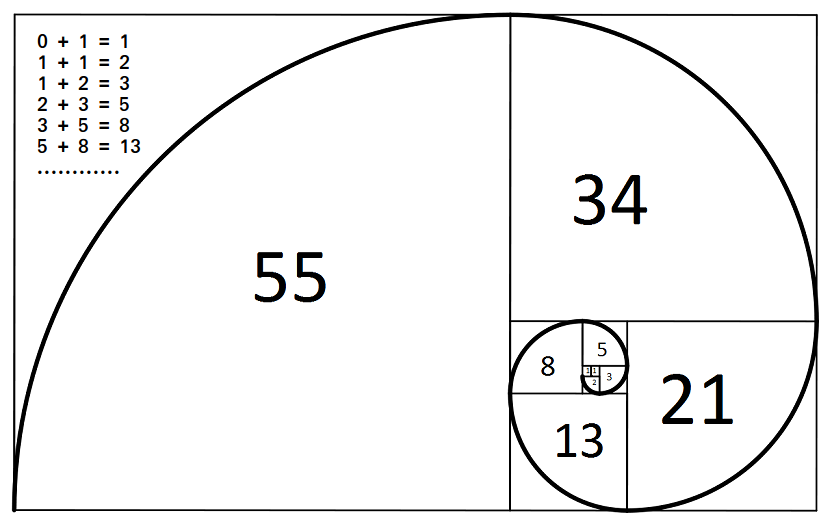
A classic example of a dynamic system of order $\mathcal{O} = 2$ is the
\begin{equation} \begin{array} \ x_1 = 0 \\ x_2 = 1 \\ x_{t} = x_{t-1} + x_{t-2} \end{array} \end{equation}This sequence naturally creates a 'golden spiral' like the one shown below (image credit).
The standard gradient descent scheme first detailed in Chapter 6 is - upon reflection - an order $\mathcal{O} = 1$ dynamic system. The way we traditionally write our gradient descent step $\mathbf{w}^k = \mathbf{w}^{k-1} - \alpha \nabla g\left(\mathbf{w}^{k-1}\right)$ tells us that the step $\mathbf{w}^{k}$ is dependent on its immediate predecessor $\mathbf{w}^{k-1}$. The momentum step (introduced in Section 13.4) then 'adds memory' to the gradient descent step, making $\mathbf{w}^{k}$ dependent on its previous $\mathcal{O} = 2$ predecessors via the update step $\mathbf{w}^k = \mathbf{w}^{k-1} - \alpha \nabla g\left(\mathbf{w}^{k-1}\right) + \beta\left(\mathbf{w}^{k-1} - \mathbf{w}^{k-2}\right)$.
The examples above - particularly Examples 4 - 6 - showcase a universal property of recurrence relations: their behavior is completely determined by their initial conditions - a fact that we easily confirm below. This is why such systems are often called chaotic: because their behavior can change dramatically based on the setting of their initial condition(s).
The behavior of a recurrence relation is completely determined by its initial condition(s).
If we closely analyze the update step for any generative dynamic system like those described above - which we will do here for an order $\mathcal{O} = 1$ system for simplicity - we can see that absolutely every point is directly related to the initial condition $x_1$. How? By 'rolling back' the system starting with the formula for $x_t$
\begin{equation} x_{t} = f\left(x_{t-1}\right) \end{equation}and then plugging in the mirroring formula for $x_{t-1}$ which is $x_{t-1} = f\left(x_{t-2}\right)$ we get
\begin{equation} x_{t} = f\left(\,f\left(x_{t-2}\right)\right). \end{equation}If we continue to roll back, substituting in the same formula for $x_{t-2}$, and then $x_{t-3}$, etc., we can eventually represent the term $x_t$ strictly in terms of $x_1$ as
\begin{equation} x_t = f\left(\,f\left(\,\cdots f\left(x_1\right)\right)\cdots\right). \end{equation}Note here we compose $f$ with itself $t$ times, and could write it more compactly as $x_t = f^{(t-1)}\left(x_1\right)$.
So indeed we can see that every point created by such a recurrence relation is completely determined by its initial condition. The same kind of relation also holds for more general order $\mathcal{O}$ systems as well.
Written text is commonly modeled as a recurrence relation. For example, take the simple sentence shown in the animation below "my dog runs". Each word in this sentence does - intuitively - seem to follow its predecessor in an orderly, functional, and predictable way. In the animation below we walk through the sentence word-by-word, highlighting the fact that each word follows its immediate predecessor just like a $\mathcal{O}=1$ dynamic system.

This kind of intuitive leap makes sense more generally as well. We can also think of each word in a sentence following logically based not just on its immediate predecessor, but several words just like an order $R$ dynamic system. Text certainly is generally structured like this - with preceding words in sentence determining those that follow.
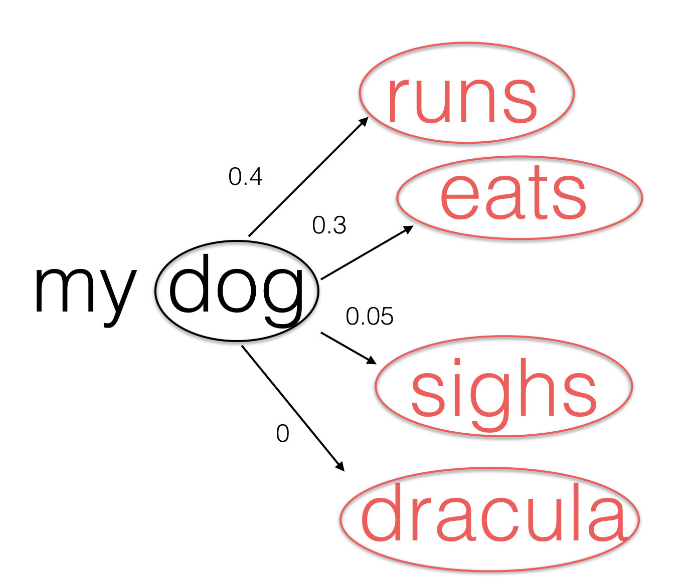
However while text certainly seems to have the structure of a dynamic system like the ones we have seen thus far, it does have one attribute that we have not seen thus far: choice. A given word does not always completely determine the word that follows it. For example, in the sentence above we could imagine a range of words following the word "dog" instead of "runs", like e.g., "eats". This would give us the sentence "my dog eats" instead of "my dog runs", which is a perfectly valid and meaningful English sentence. Of course there are other words that could follow "dog" as well, some of which like e.g., the word "sighs" that while valid would be less common than "eats". However some words, like e.g., "dracula", making the sentence "my dog dracula" do not make any sense at all.

So in summary, while a valid sentence of English words clearly has ordered structure like a dynamic system, with each word following its predecessor, there are often many choices for subsequent words (unlike the dynamic systems we have seen previously). Moreover of the choices following a particular word we can reasonably say that some are more likely to occur than others. In other words, these choices are stochastic in nature (stochastic means choices) - with each having a different probability of occurring. For example, below we show the four choices of words following "dog" in the sentence above assigning (using our intuition) a probability of occurring to each. Here we suppose the word "runs" is the most probable, "eats" the next, and so on.
The probabilities shown do not add up to $1$ because there could be other reasonable words that could follow "dog" other than those shown here. To more accurately estimate these probabilities - and to identify all of the other possible words that follow "dog" - it is common to take a large body of text (like e.g., a long book), scan it for all occurrences of the word "dog" and make a listing of all the words following it along with their frequency. Then to create a sample probability for each - so that the sum of the probabilities adds up to $1$ - we simply divide off the total number of times "dog" appeared in the text (often referred to as a corpus).
Irregardless of how we compute the probabilities, mathematically speaking we codify the list possible outputs and their probability of occurrence - like the list of possible words shown above following "dog" - as a histogram (which is often also called a probability mass function). This is just a mathematical function with many possible outputs to a single input, each weighted with its respective probability $\mathscr{p}$. For example, we can formally write the histogram of possible outputs of words following "dog" as
Here in each case '$p$' stands for the probability of the corresponding word occurring. Our prediction for the next word in the sentence is then simply the one that is most valuable, or the one with the largest probability. Here suppose that word is "runs". Translating this statement into math, we predict the word following "dog" by taking the $\text{argmax}$ over all of the choices above as
More generally, if we denote by $x_{t-1}$ the $\left(t-1\right)^{th}$ word in a sentence, and $u$ any particular word than the probability $\mathscr{p}$ above of $x_{t}$ occuring (following $x_{t}$) (often called the transition probability) than the histogram can be written more generally as
\begin{equation} \text{histogram}\left(x_{t}\right) = u \,\,\,\,\text{with probability} \,\,\,\mathscr{p}. \end{equation}Then the choice of the next word $x_{t}$ can likewise be written in general as
\begin{equation} x_{t} = \underset{\mathscr{p}}{\text{argmax}}\,\, \text{histogram}\left(x_{t-1}\right). \end{equation}We can perhaps now see how this model of written text is indeed a dynamic system. If we in general denote
\begin{equation} \underset{\mathscr{p}}{\text{argmax}}\,\, \text{histogram}\left(x_{t-1}\right) = f\left(x_{t-1}\right) \end{equation}and the first word in a sentence as $x_1 = \gamma$. Then the order $\mathcal{O} = 1$ model of text we have detailed above does indeed fit the pattern of a recurrence relation as
\begin{array} \ x_1 = \gamma \\ x_{t} = f\left(x_{t-1}\right). \end{array}We could then likewise define general order $\mathcal{O}$ model as well. Here the $t^{th}$ update would depend on its $\mathcal{O}$ predecessors but be similarly defined as
\begin{equation} x_{t} = f\left(x_{t-1},...,x_{t-\mathcal{O}}\right). \end{equation}Regardless of order, this kind of dynamic system is often called a Markov Chain.
In this example we generate a Markov chain model of text using the classic novel War of the Worlds by H.G. Wells to define our transition probabilities. Below we print out the first $500$ characters of the novel. Note some pre-processing has been done here - in particular we removed any strange characters introduced when converting this book to its e-version, and lower-case-afied all alphabetical characters.
Using an order $\mathcal{O} = 1$ model we then pick a word randomly from the text, and start generating text. Below we compare a chunk of $30$ words from the text following this initial input, and below it we show the result of the Markov model. Here the input word $x_1 = \gamma$ is colored red, and the $30$ words generated using it are colored blue. Note this means that we first plug in the word "had" into our model, which returns the word "been". Then we return "been" and it returns "the", etc.,
Clearly we can see that the Markov model, having only a single word in the past to base the next word on, does not generate anything meaningful. However as we increase the order to e.g., $\mathcal{O} = 2$ we can see that the generated sentence starts to make more sense, matching its original as shown below. Here the two initial words are colored red, with the remaining generated words colored blue. Notice this means that we first plug in the first two words (here the phrase "trucks bearing") and it returns "huge", then we plug in the next two words (here "bearing huge") and it returns "guns", etc.,
As we increase the order $\mathcal{O}$ of the model the generated text will begin to match the original more and more. For example, by the time we crank up the order to $\mathcal{O} = 10$ the text generated by the model is identical to the original.
Why does this happen? Notice that when we increase the order of the model the number of unique input sequences proliferates rapidly. Eventually, when we increase the order enough, there remains only a single exemplar (input/output pair) in the text to construct each associated histogram (i.e., every input sequence used to determine the transition probabilities is unique). Past this point we only have a single example of each input, thus only one choice for its associated output: whatever follows it in the text (with probability $\mathscr{p} = 1$).
Just modeled text by words above using a Markov chain, we can likewise model it via characters. For the same intuitive reasons as discussed in the context of the text-wise modeling scheme - characters often logically follow one another in succession - we can model text as a stochastic dynamic system (a Markov chain) over characters as well.
Below we show the result of an order $\mathcal{O} = 1$ Markov chain model using the characters instead of words, and the same text (H.G. Well's classic War of the Worlds) to calculate our transition probabilities. Of course using only a single character as precedent we cannot capture much about the text, as reflected in the generated text below. Here the single character used as input is colored red, with $300$ generated characters using the order $1$ model colored blue. Note that this means that the first character "n" is plugged into the model and returns the second, here the space character. This is then plugged in to generate "t", etc.,
As we saw in the previous example, as we increase the order $\mathcal{O}$ of the model we capture more and more about the text, and can therefore generate more and more meaningful sentences. For example, below we show the result of an order $\mathcal{O} = 5$ model, comparing to the similar chunk of the true text. With this many characters we actually start to generate a number of real words.
Increasing the order $\mathcal{O} = 10$ we can further observe this trend.
Finally, just as in the word generating case, if we increase the order $\mathcal{O}$ past a certain point our model will generate the text exactly. Below we show the result of an order $\mathcal{O} = 50$ model, which generates precisely the true text shown above it. This happens for exactly the same reasoning given previously in the context of the word based model: as we increase the order of the model the number of unique input sequences balloons rapidly, until each input sequence of the text is unique. This means that there is only one example of each used to determine the transition probabilities, i.e., precisely the one present in the text.
From the very definition of an order $\mathcal{O} = 1$ system - with generic update step given as
\begin{equation} x_{t} = f\left(x_{t-1}\right) \end{equation}we can see that each $x_{t}$ is dependent on only the value $x_{t-1}$ that comes before it, and no prior point (like e.g., $x_{t-2}$). Likewise an order $\mathcal{O}$ system with generic update steps
\begin{equation} x_{t} = f\left(x_{t-1},\,...,x_{t-\mathcal{O}}\right) \end{equation}says that the update for any $x_{t}$ is only on dependent $x_{t-1}$ through $x_{t-\mathcal{O}}$, and no point coming before $x_{t-\mathcal{O}}$. So - regardless of order - the range of values used to build each subsequent step is limited by the order of the system.
The consequence of such systems being limited by their order is perhaps most clearly seen by a simple example of a Markov chain model of text. For example, suppose we have constructed a word-based Markov model of order $\mathcal{O} = 1$, whose transition probabilities have been determined using a large text corpus. We the apply our model to both of the sentences shown below, to predict the word following "is".
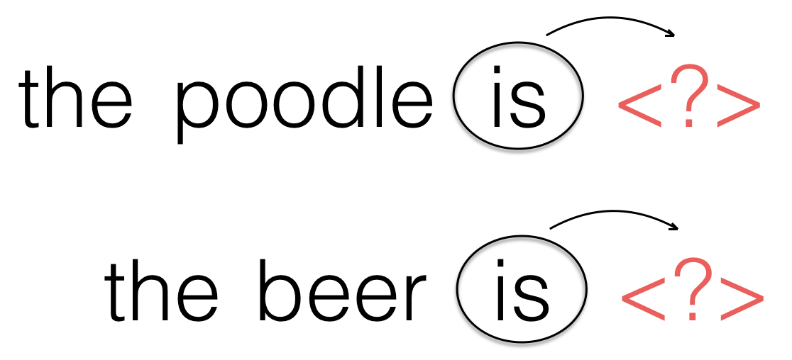
The problem here is that - because we have used an order $\mathcal{O} = 1$ model - the same word will be predicted to follow the word "is" in both sentences. This will likely mean that at least one (if not both) of the completed sentences will not make sense, since they have completely different subjects. Because a fixed order dynamic system is limited by its order, and cannot use any information from earlier in a sequence, this problem can arise regardless of the order $\mathcal{O}$ we choose.