code

share


Reinforcement Learning (RL) is a general machine learning framework for building computational agents which can, if trained properly, act intelligently in a complex (and often dynamic) environment in order to reach a narrowly-defined goal. Interesting applications of this framework include game AI (e.g., AlphaGo, chess, self-playing Atari and Nintendo games), as well as various challenging problems in automatic control and robotics.
Understanding the full blown modern use of Reinforcement Learning can be challenging due to the sheer number of complex ideas involved. Further complicating matters, Reinforcement Learning almost always requires the use of advanced ideas from machine learning (e.g., features, mathematical optimization, and deep neural networks) for satisfactory performance. Together these factors make Reinforcement Learning a rather tough subject to learn for the first time.
In this series of notebooks we introduce Reinforcement Learning by pulling apart the entire process, and by introducing each concept as it is needed. By focusing our attention on just one piece of the system at-a-time we can gain a fuller understanding of how each component works, and why it is needed. Moreover by doing so we also gain some extremely important but surprisingly uncommon intuition about how the individual components of Reinforcement Learning define the strengths and limitations of the process in general.
We begin our discussion of the RL framework by first describing some of its common applications from three main areas in which Reinforcement Learning is commonly used: robotics, game AI, and automatic control. These example applications represent the kind of tasks that can be automated using the Reinforcement approach. We will return to these examples repeatedly throughout this series as we develop RL concepts.
Path planning problems are commonly encountered in robotics applications, as well as video games, and mapping services. For many robots (e.g., a cleaning bot) path planning is essential for efficient operation. In a video game the enemy AI uses path planning to reach human players in a level as quickly as possible. With a digital mapping service, path planning is used to efficiently route you from point A to point B [2].
We will look, throughout the RL series, at a toy version of this problem called Gridworld, wherein the robot (agent) must learn how to navigate a grid-like map efficiently in order to reach a target destination (goal) on the map. Figure below shows a simple example of Gridworld - a small maze. The blue square here denotes the robot's location and the green square the desired destination. In the Gridworld environment the robot can move one unit left, right, up, or down at a time, to any ‘safe’ square (colored gray). While the robot is also allowed to pass through the ‘hazard’ squares (colored red), it would be heavily penalized for doing so, as these squares simulate hazardous locations, e.g., a slippery or obstructed part of the floor. Starting at any given location, the agent in Gridworld must learn the shortest path to the green square while avoiding hazards along the way.
Note that in Gridworld the agent cannot ‘see’ the entire map, the way it is depicted in the figure above. From the agent’s perspective, the world looks like the one shown below where the robot can only see those parts of the map it is allowed to move to.
Gridworlds come in many shapes and sizes. Here is one example where the hazards are arranged in a certain way to form a narrow passage of safe squares separating one half of the world from another. If the robot starts on the ‘wrong’ side of the world, as shown below, then it must cross a narrow bridge of safe squares to reach the target.
Another example: a Gridworld with randomly-placed hazards! In this case too, the robot must learn to navigate a hazard-free path to reach the target efficiently.
Another common application of Reinforcement Learning is to train AI agents to win certain games. In the game of chess for example, this means training an agent that can consistently check-mate its opponent [3].
Reinforcement Learning can also be used to train an agent to win (simple) video games, like those from the Atari 2600 collection [4], and Pac-Man [5].
Many automatic control problems involve teaching an agent how to control a particular mechanical, electrical, or aerodynamic system. One classic toy example in this area is to teach an agent how to balance a pole on a moving cart, sometimes referred to as the cart-pole or inverted pendulum problem. The pole is free to rotate about an axis on the cart, with the cart on a track so that it may be moved left and right, affecting the location of the pole. The pole feels the force of Earth's gravity, and so if unbalanced, will fall to the ground [6].
Autopilot systems are another technology that can make use of Reinforcement Learning. A toy problem in this area is the so-called lunar-lander, where the objective is to simulate a real lunar lander by training an RL agent that can correctly land a space craft in a certain landing zone (in the area between the two flags as shown in the figure below) [6].
The applications we discussed in the previous section, while seemingly quite different, share a common element: they all have narrowly-defined goals that the Reinforcement agent is trained to accomplish. With the autopilot system on an airplane for instance, the goal is to keep the plane flying safely towards towards a pre-defined destination. To achieve this goal, one could attempt to collect and code up a list of if-then rules to solve this problem. However, the sheer amount of sensory data that must be factored in when compiling the list (plane's velocity, altitude, ambient air pressure, stress on various parts of the vehicle, etc.) would extremely complicate the process. Additionally, there are a myriad of environmental factors to deal with (e.g., air density, wind velocity and currents) that can vary wildly from flight to flight.
The Reinforcement approach ditches the notion of producing a long list of engineered conditionals to solve such a problem, and instead trains a computational agent to accomplish the desired goal. To do this, the agent must have the ability to experiment in the actual space of a given problem, or a realistic simulation of the problem environment. Therefore it must have knowledge of the problem environment (or simulator) during the learning process. This information is given to the agent, through what is called state in the RL jargon.
A state is a variable that communicates characteristic information about the problem environment to the agent.
But how does the agent learn as it interacts with the problem environment? The same way humans do when we are thrown into a new environment - one in which we have no theory or principles to stand on - by repeated trial and error interactions. For example in the case of an autopilot system, we would train an RL agent by giving it control of an airplane in a simulated environment. We would then run many simulations of the airplane traveling in various conditions, in each simulation giving the agent full control over steering the airplane. At first the agent makes random steering actions, likely crashing the plane and ending the simulation. After many rounds of this type the agent slowly starts learning how to steer correctly to achieve the goal of reaching a pre-defined destination point.
In navigating the problem environment in pursuit of the desired goal, the RL agent takes a sequence of actions in a trial-and-error fashion.
Of crucial importance here is the fact that it is the entire sequence of actions taken together that we want to lead successfully to accomplishing the goal. This very fact makes Reinforcement Learning inherently more challenging than supervised learning problems like regression and classification. The following quote from [1] nicely summarizes this challenge:
"Reinforcement learning is a difficult problem because the learning system may perform an action and not be told whether that action was good or bad. For example, a learning auto-pilot program might be given control of a simulator and told not to crash. It will have to make many decisions each second and then, after acting on thousands of decisions, the aircraft might crash. What should the system learn from this experience? Which of its many actions were responsible for the crash? Assigning blame to individual actions is the problem that makes reinforcement learning difficult."
This brings us to an important question: how can we communicate an abstract goal (like reach destination safely) to the agent, so it can learn through many simulations the correct sorts of actions to take? In the RL framework we translate the desired goal into a series of numerical values called rewards. These reward values provide feedback to the agent at each step of a simulation run. Essentially they tell the agent how well it is accomplishing the desired goal, helping the agent eventually learn the correct sequence of actions necessary to achieve it.
A reward is a numerical value given to the RL agent after it takes an action, to communicate to the agent whether we think the taken action has helped or hindered its accomplishment of the desired goal.
Note that it is completely up to us (humans) to decide on the reward structure. Intuitively, we want a reward for a given action to be larger for those actions that get us closer to accomplishing our goal (and less for those actions which do not). Designing a good reward structure is therefore crucial in solving any Reinforcement Learning problem as this is the (only) way we communicate our desired goal to the agent.
States, actions, and rewards are three fundamentals concepts in Reinforcement Learning that connect together to create a feedback system that, when properly engineered, allow us to train an RL agent to accomplish a task. The agent based on the feedback it receives during training via our designed reward structure, learns how to take reward-maximizing actions that eventually lead to the desired goal. To further conceptualize these fundamental ideas, we now give several examples using the RL applications introduced in the previous section.
For any given Gridworld, knowledge of the agent’s current location is enough to fully describe the problem environment. Hence, a state in this case consists of the horizontal and vertical coordinates of the blue square on the map. Recall that the robot in Gridworld is only allowed to move one unit up, down, left or right. These define the set of actions that the Gridworld agent can take. Note that depending on the agent’s location (state), only a subset of actions may be available to the agent. For instance if the agent is at the top left corner of the map, it will only be allowed to go one unit right or down.
We can design a variety of reward structures to communicate our goal to the agent, that is, to reach the target (green square) in an efficient manner while avoiding the hazards (red squares). For example, we can assign a negative value like -1 to all actions (one unit movement) which lead to a non-goal and non-hazard state, a larger negative value like -100 for those actions leading to a hazard state, and a non-negative number like 0 to actions leading to the goal state itself. This way, the agent is incentivized not to step on hazard squares (as its reward will be reduced by 100 each time it does so), and to reach the goal state in as few steps as possible (since walking over each white square still reduces its reward by 1).
To summarize, beginning at a state (location) in Gridworld, an action is taken to move the agent to a new state. For taking this action and moving to the new state the agent receives a reward.
In the chess problem a state is any (legal) configuration of all (remaining) white and black pieces on the board, and an action is a legal move of any of current pieces on the board according to the rules of chess. In this case one reward structure to induce our agent to learn how to win could be as follows: any move made that does not immediately lead to the goal state (checkmating the opponent) receives a -1 reward, while a move that successfully check mates the opponent receives a large positive reward (of 10,000 for instance).
In the cart-pole problem a state is a complete set of information about the cart and pole's position. This includes the cart position, the cart velocity, the angle of the pole measured as its deviation from the vertical position, and the angular velocity of the pole. While these are technically continuous values, in practice they are finely discretized. Note that in order to solve the cart-pole problem in an RL framework we need not make any assumptions about the environment, e.g., the fact that gravity exists, its precise force, etc.
The range of actions in the cart-pole example is completely defined by the available range of motions of the machine being directly controlled. In our toy example the agent can keep the cart still or move it one unit to the left or right along the horizontal axis. One common choice of reward structure in this case: at every state at which the angle between the pole and the horizontal axis is above a certain threshold the reward is 1, otherwise it is 0. Therefore beginning at a state (a specific configuration of the four system descriptors mentioned above) an action is taken (the cart is kept still or moved), and a new state of the system arises. For taking this action and moving to the new state the agent receives a reward.
Now that you are familiar with the fundamental concepts of RL (states, actions, and rewards), it is time to introduce notation that will allow us to represent each of these concepts algebraically. Suppose for now, that any given problem only has a finite number of states and actions. We will denote the set of all states by $S=\left\{ \sigma_{1},\sigma_{2},...,\sigma_{N}\right\}$, and the set of all actions by $A=\left\{ \alpha_{1},\alpha_{2},...,\alpha_{M}\right\}$.
At the $k^{th}$ step in solving an RL problem, the agent begins at a state $s_{k} \in S$, takes an action $a_k \in A$ that moves the system to a state $s_{k+1} \in S$. Be careful not to confuse the $s$'s with the $\sigma$'s, and the $a$'s with the $\alpha$'s. The notation $s_{k}$ is a variable denoting the state at which the $k^{th}$ step of the procedure begins, and so can be any of the possible realized states in $S=\left\{ \sigma_{1},\sigma_{2},...,\sigma_{N}\right\}$. Likewise the notation $a_k$ is a variable denoting the action taken at the $k^{th}$ step, which is one of the permissible actions from $A=\left\{ \alpha_{1},\alpha_{2},...,\alpha_{M}\right\}$.
Recall that the mechanism by which an agent learns the best action to take in a given state is the reward structure. So we also need notation for the reward an agent receives at the $k^{th}$ step as well: call this $r_k$. This is a function of the initial state at this step the action taken, i.e., $r_k = r_k(s_{k},a_k)$.
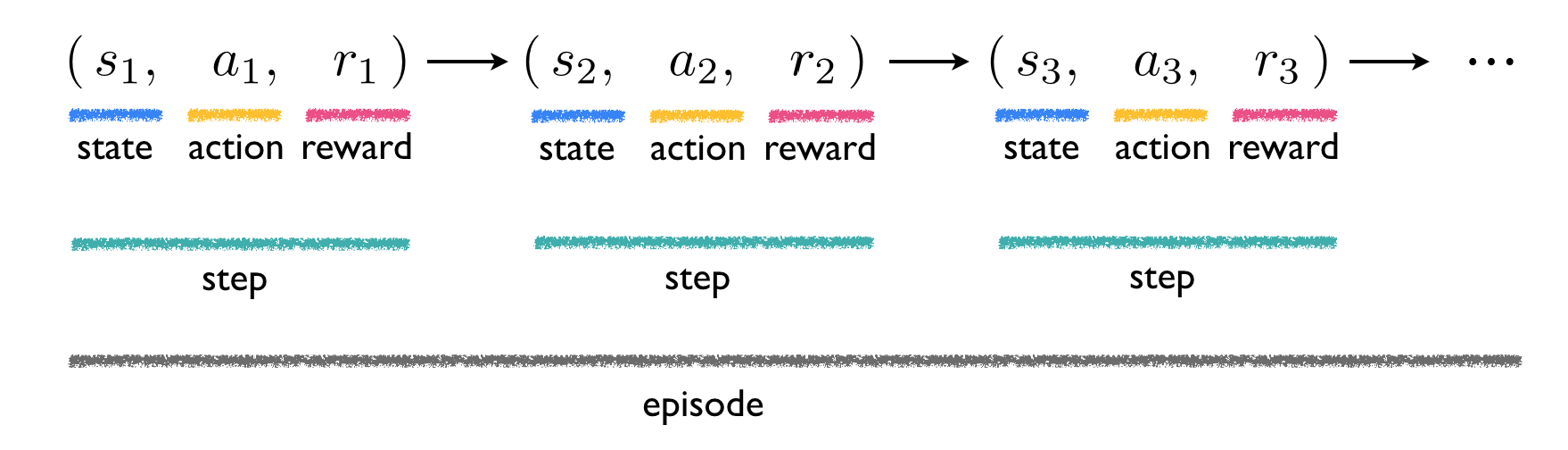
To reiterate, in solving an RL problem an agent goes through a sequence of events at each step. These are: start at a state, take an action, move to a new state, and receive a corresponding reward. The first three steps therefore look like
Step 1
Step 2
Step 3
Taken together a sequence of such steps, ending either when a goal state is reached (as in the Gridworld or chess examples) or after a maximum number of iterations is completed (as in the cart-pole example), is referred to in RL jargon as an episode. The RL nomenclature and notation introduced so far are summarized in the figure below.
We end this brief section by noting that not all RL problems are deterministic in nature, such as those considered here, where one realized action $a_k$ at a given state $s_k$ always leads to the same next state $s_{k+1}$. In stochastic RL problems, a given action at a state may lead to different conclusions. For example, many RL-based robotics problems are stochastic in nature: a robot may perform a given action - like accelerate forward one unit of thrust - at a state and reach different outcomes due to things like inconsistencies in the application of this action, sensor issues, friction, etc. Almost the same modeling used above captures this variability for such stochastic problems, with the main difference being that the reward function must also necessarily be a function of the state $s_{k+1}$ in addition to $s_k$ and $a_k$. We will deal this generality later on once we flush out all the details of the deterministic scenario.
With notation out of the way, we are now ready to address perhaps the most important question in Reinforcement Learning: how do we train the agent? The answer is, like any other machine learning problem, through optimizing an appropriate cost function. However, unlike other machine learning problems such as linear or logistic regression, we cannot directly work out an exact parameterized form of the cost function here. Instead what we can do is formalize a certain attribute we want this function to ideally have and, working backwards, we can arrive at a method for computing it. In what follows we do exactly this, noting that with Reinforcement Learning we ideally want the agent to learn to take proper actions at each state that its total reward.
Define $Q(s_1,a_1)$ as the maximum total reward possible if we begin at a state $s_1$, take the action $a_1$, and then continue taking steps until the goal is reached or a maximum number of steps is taken. Now recall that taking the action $a_1$ brings us to some state $s_2$ and the agent receives some reward $r_1$. Therefore $Q(s_1,a_1)$ can be calculated as the sum of the realized reward $r_1$ plus the largest possible total reward from all the proceeding steps starting this time from the state $s_2$. Invoking the definition of $Q$, this latter quantity can be written as
$\underset{i\in\varOmega(s_2)}{\text{maximum}}\,\,Q\left(s_{2},\,\alpha_{i}\right)$
where $\varOmega(s_2)$ denotes the index set for all valid actions that can be taken when the agent is at the state $s_2$. Writing out the equality above algebraically, we then have
$Q\left(s_{1},\,a_{1}\right)=r_{1}+\underset{i\in\varOmega(s_2)}{\text{maximum}}\,\,Q\left(s_{2},\,\alpha_{i}\right)$
Note that the expression above holds regardless of what state and action we begin with. That is, at the $k^{th}$ step, we can write
$Q\left(s_{k},\,a_{k}\right)=r_{k}+\underset{i\in\varOmega(s_{k+1})}{\text{maximum}}\,\,Q\left(s_{k+1},\,\alpha_{i}\right)$
This recursive definition of the $Q$ function is typically referred to as Bellman's equation. In the next post we discuss, in full detail, how to resolve the $Q$ function, or in other words train the RL agent, via the so-called Q-Learning algorithm.
The content of this notebook is supplementary material for the textbook Machine Learning Refined (Cambridge University Press, 2016). Visit http://mlrefined.com for free chapter downloads and tutorials, and our Amazon site for details regarding a hard copy of the text.
[1] Mance Harmon and Stephanie Harmon. Reinforcement Learning: A Tutorial. No. WL-TR-97-1028. Wright Lab Wright-Patterson AFB OH, 1997
[2] There are many algorithms specifically designed to solve just this task - the most popular being Dijkstra’s and A* algorithms. However the more flexible RL framework too provides great results.
[3] Matthew Lai. Giraffe: Using deep reinforcement learning to play chess. arXiv:1509.01549 (2015).
[4] Volodymyr Mnih et al. Playing atari with deep reinforcement learning. arXiv:1312.5602 (2013).
[5] Image taken from http://ai.berkeley.edu/project_overview.html
[6] Image taken from https://gym.openai.com/