In this part of the text (Chapters 5 - 7) we take our first step into discussion mathematical optimization, a collection of algorithmic tools designed to find the smallest points (called minima) of a mathematical function. Why discuss such technical matters prior to discussing machine learning / deep learning models themselves? Because mathematical optimization is the absolute workhorse of machine learning and deep learning, it is the set of algorithmic tools we use to make our machine learning / deep learning models actually learn from data.

Thankfully - much like calculus, statistics, and linear algebra - much of the thrust of mathematical optimization can be discussed off-line and - even better - can be illustrated beautifully using simple visual and geometric examples. By confronting these technical matters now - prior to diving into the sophisticated details of learning models - we can better prepare ourselves to deal with the broader learning processes, since mathematical optimization is intimately involved in nearly every machine learning / deep learning problem.

5.0.1 Mathematical optimization and machine learning / deep learning

Every machine learning / deep learning learning problem has parameters that must be tuned properly to ensure optimal learning. For example, there are two parameters that must be properly tuned in the case of a simple linear regression - when fitting a line to a scatter of data: the slope and intercept of the linear model.

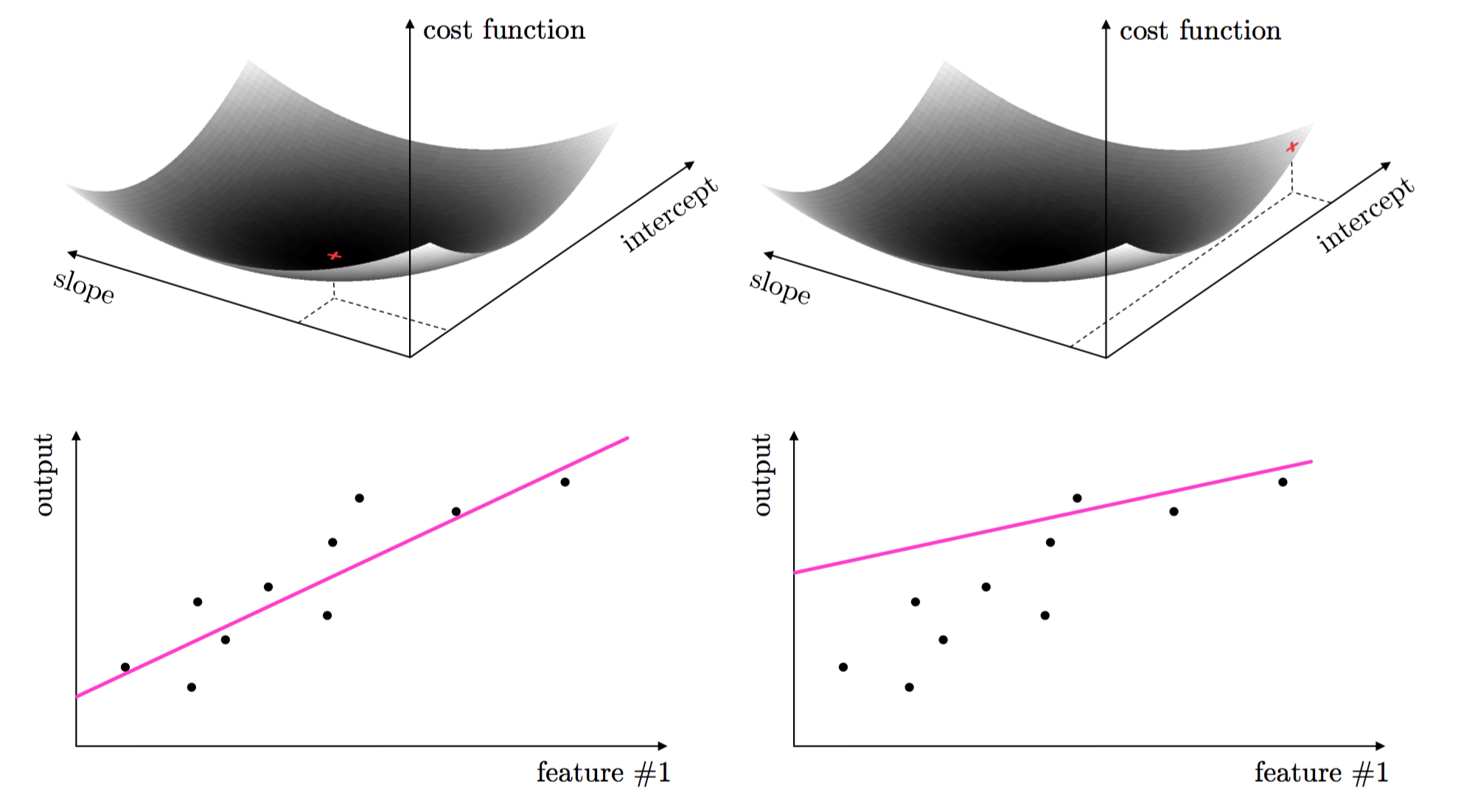
These two parameters are tuned by forming what is called a cost function or loss function. This is a continuous function in both parameters - that measures how well the linear model fits a dataset given a value for its slope and intercept. The proper tuning of these parameters via the cost function corresponds geometrically to finding the values for the parameters that make the cost function as small as possible or, in other words, minimize the cost function. The image below - illustrates how choosing a set of parameters higher on the cost function results in a corresponding line fit that is poorer than the one corresponding to parameters at the lowest point on the cost surface.

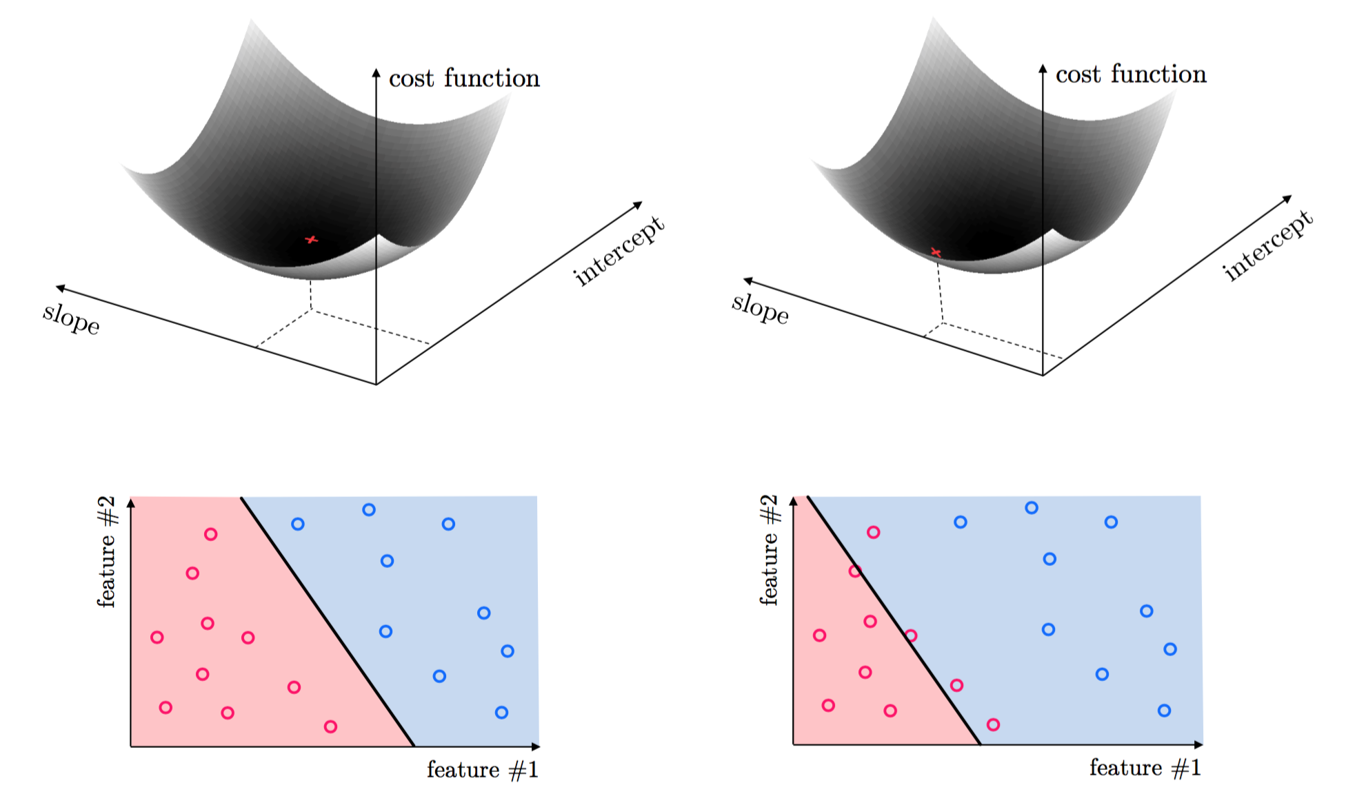
This same idea holds true for regression with higher dimensional input, as well as classification where we must properly tune parameters to separate classes of data. Again, the parameters minimizing an associated cost function provide the best classification result. This is illustrated for classification below.

The tuning of these parameters require the minimization of a cost function can be formally written as follows. For a generic function $g(\mathbf{w})$ taking in a general $N$ dimensional input $\mathbf{w}$ the problem of finding the particular point $\mathbf{v}$ where $g$ attains its smallest value is written formally as

\begin{equation} \underset{\mathbf{w}}{\mbox{minimize}}\,\,\,\,g\left(\mathbf{w}\right) \end{equation}

As detailed in our series on the vital elements of calculus, the first order optimality condition characterizes solutions to this problem. However because these conditions can very rarely be solved 'by hand' we must rely on algorithmic techniques for finding function minima (or at the very least finding points close to them). In this part of the text we examine many algorithmic methods of mathematical optimization, which aim to do just this.

The tools of mathematical optimization are designed to minimize cost functions. When applied to learning problems this corresponds to properly tuning the parameters of a learning model. Mathematical optimization is the workhorse of machine learning / deep learning, playing a role in virtually every learning problem.