Chapter 12: Introduction to nonlinear learning

12.1 Features, functions, and nonlinear regression

In this Section we introduce the general framework of nonlinear regression, along with many examples ranging from toy datasets to classic examples from differential equations.

These examples are all low dimensional, allowing us to visually examine patterns in the data and propose appropriate nonlinearities, which we can (as we will see) very quickly inject into our linear supervised paradigm to produce nonlinear regression fits.

y walking through these examples we flush out a number important concepts in concrete terms, coding principles, and jargon-terms in a relatively simple environment that will be omnipresent in our discussion of nonlinear learning going forward.

Activate next cell to toggle code on and off

from IPython.display import display
from IPython.display import HTML
import IPython.core.display as di # Example: di.display_html('<h3>%s:</h3>' % str, raw=True)

# This line will hide code by default when the notebook is eåxported as HTML
di.display_html('<script>jQuery(function() {if (jQuery("body.notebook_app").length == 0) { jQuery(".input_area").toggle(); jQuery(".prompt").toggle();}});</script>', raw=True)

# This line will add a button to toggle visibility of code blocks, for use with the HTML export version
di.display_html('''<button onclick="jQuery('.input_area').toggle(); jQuery('.prompt').toggle();">Toggle code</button>''', raw=True)

Toggle code

12.1.1 Modeling principles of linear regression

• linear regression begins with a very particular ideal desire to relate the input/output linearly

\begin{equation} w_0 + x_{1,p}w_1 + \cdots + x_{N,p}w_N \approx y_p \end{equation}

• when these weights were tuned properly they all lie close to a particular hyperplane defined by the ideal weights.

• our linear predictor or model

\begin{equation} \text{model}\left(\mathbf{x},\mathbf{w}\right) = w_0 + x_{1}w_1 + \cdots + x_{N}w_N \end{equation}

or more compactly

\begin{equation} \text{model}\left(\mathbf{x},\mathbf{w}\right) = \mathbf{x}^T \mathbf{w}^{\,} \end{equation}

where we use our 'compact' notation denoting

\begin{equation} \mathbf{w}=\begin{bmatrix} w_{0}\\ w_{1}\\ w_{2}\\ \vdots\\ w_{N} \end{bmatrix} \,\,\,\,\,\,\,\,\,\,\,\,\,\,\,\,\,\,\,\,\,\,\,\,\,\,\,\,\,\,\,\, \mathbf{x}=\begin{bmatrix} 1 \\ x_{1}\\ w_{2}\\ \vdots\\ w_{N} \end{bmatrix},\,\,\,\, \end{equation}

• the linear model compactly in Python

# compute linear combination of input point
def model(x,w):
    # tack a 1 onto the top of each input point all at once
    o = np.ones((1,np.shape(x)[1]))
    x = np.vstack((o,x))
    
    # compute linear combination and return
    a = np.dot(x.T,w)
    return a

• in our model notation our ideal linear relationship

\begin{equation} \text{model}\left(\mathbf{x}_p, \mathbf{w}\right) \approx y_p. \end{equation}

• to tune properly square the difference and sum over all points

\begin{equation} g\left(\mathbf{w}\right) = \frac{1}{P}\sum_{p=1}^{P}\left(\text{model}\left(\mathbf{x}_p,\mathbf{w}\right) - y_p\right)^2 \end{equation}

• minimum provides us with the weights that service our ideal as best as possible

Example 1. The 'perfect' dataset for linear regression

• in a perfect world our desired approximations $\approx$ can attain a strict equality $=$ i.e.,

\begin{equation} \text{model}\left(\mathbf{x}_p,\mathbf{w}\right) = y_p \end{equation}

• in such a perfect instance the dataset lies precisely on a line (or more generally, a hyperplane)

12.1.2 Modeling principles of general nonlinear regression

• to generalize our regression paradigm to nonlinear case - swap out the linear model used in the construction of our regression

• beginning with the ideal scenario in equation, where we suppose we have perfect weights and ending with the Last Squares cost function in equation for recovering them, there was nothing particular to this argument demanded that our model be a linear one

• this was an assumption we made - we chose a linear model to perform regression with.

• so instead of using a linear model we could instead use a nonlinear one, involving a single nonlinear function $f$

\begin{equation} \text{model}\left(\mathbf{x},\mathbf{w}\right) = w_0^{\,} + {w}_{1}^{\,}\,f\left(\mathbf{x}_p\right). \end{equation}

• note here $\mathbf{w}$ contains weights of linear combination and any internal weights of $f$

• in the jargon of machine learning / deep learning the nonlinear function $f$ is often called a nonlinear feature transformation, since we it transforms our original input features $\mathbf{x}$

• again we could consider the ideal case - where we have knowledge of the best possible weights so that

\begin{equation} \text{model}\left(\mathbf{x}_p,\mathbf{w}\right) \approx y_p \end{equation}

• the same logic leads us to learn these parameters via minimizing e.g., a Least Squares cost function

\begin{equation} g\left(\mathbf{w}\right) = \frac{1}{P}\sum_{p=1}^{P}\left(\text{model}\left(\mathbf{x}_p,\mathbf{w}\right) - y_p\right)^2 \end{equation}

• minimum will recover our desired weights

• in general we can form a nonlinear model that is the weighted sum of $B$ nonlinear functions of our input as

\begin{equation} \text{model}\left(\mathbf{x},\mathbf{w}\right) = w_0 + {w}_{1}\,f_1\left(\mathbf{x}_p\right) + {w}_{2}\,f_2\left(\mathbf{x}_p\right) + \cdots + w_B\,f_B\left(\mathbf{x}_p\right) \end{equation}

where $f_1,\,f_2,\,...\,f_B$ are nonlinear parameterized or unparameterized functions - or feature transformations

• $w_0$ through $w_B$ (along with any additional weights internal to the nonlinear functions) are represented in the weight set $\mathbf{w}$ and must be tuned properly

• we tune this model via the same steps as before, forming e.g., a Least Squares cost and minimizing

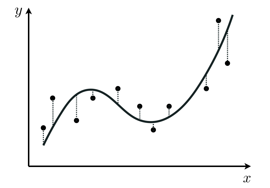
Example 2. The perfect dataset for nonlinear regression

• in complete analogy to the linear case, here our perfect dataset would consist of points where

\begin{equation} \text{model}\left(\mathbf{x}_p, \mathbf{w}\right) = y_p \end{equation}

• i.e., points lying perfectly on the nonlinear curve (or in general the nonlinear surface) defined by $f$.

12.1.3 Introductory examples of nonlinear regression

• here we walk through a number of simple examples of nonlinear regression where we can determine - by eye - a proper nonlinear model

• doing this helps flush out a number of mathematical and programming concepts that are crucial going forward

• first up: its time to officially abstract our cost function(s) for regression e.g., Least Squares

# an implementation of the least squares cost function for linear regression
def least_squares(w):
    cost = np.sum((model(x,w) - y)**2)
    return cost/float(len(y))

• this works regardless of the model - linear or nonlinear - so we can push it to the back

• we can also abstract our model function too, since will look essentially the same throughout all examples

• with the inclusion of general feature transformation(s) our model will always look like

# an implementation of our model employing a nonlinear feature transformation
def model(x,w):    
    # feature transformation 
    f = feature_transforms(x,w[0])
    
    # tack a 1 onto the top of each input point all at once
    o = np.ones((1,np.shape(f)[1]))
    f = np.vstack((o,f))
    
    # compute linear combination and return
    a = np.dot(f.T,w[1])
    return a

• here f = feature_transforms(x,w[0]) computes our desired feature transformations

• compare to our original model implementation - just a few lines extra to compute features

# compute linear combination of input point
def model(x,w):
    # tack a 1 onto the top of each input point all at once
    o = np.ones((1,np.shape(x)[1]))
    x = np.vstack((o,x))
    
    # compute linear combination and return
    a = np.dot(x.T,w)
    return a

• so we can abstract model as well, since it will always look similar regardless of linear/nonlinear features

• in short then, we just need to worry about implementing our feature_transforms in Python

• once defined we can then feed into model, and feed model into e.g., least_squares to optimize

Example 3. The linear case

• as a first and simple example we can write the feature_transforms function for the simple case of linear regression

## This code cell will not be shown in the HTML version of this notebook
# load data
csvname = datapath + 'unnorm_linregress_data.csv'
data = np.loadtxt(csvname,delimiter = ',')

x = data[:,:-1].T
y = data[:,-1:] 

# plot dataset
demo = regress_plotter.Visualizer(data)
demo.plot_data()

• employ simple linear feature transformation

\begin{equation} f\left(x\right) = x \end{equation}

and in this notation our model is then equivalently

\begin{equation} \text{model}\left(x,\mathbf{w}_{\!}\right) = w_0 + w_{1\,}f\left(x\right). \end{equation}

# the trivial linear feature transformation
def feature_transforms(x):
    return x

## This code cell will not be shown in the HTML version of this notebook
# pluck out best weights - those that provided lowest cost, 
# and plot resulting fit
ind = np.argmin(run.cost_history)
w_best = run.weight_history[ind]
demo.plot_fit(w_best,run.model,normalizer = run.normalizer);

Example 4. Modeling a familiar wave using a parameterized feature transformation

## This code cell will not be shown in the HTML version of this notebook
# load data
csvname = datapath + 'noisy_sin_sample.csv'
data = np.loadtxt(csvname,delimiter = ',')
x = data[:,:-1].T
y = data[:,-1:] 

# plot dataset
demo = regress_plotter.Visualizer(data)
demo.plot_data()

• completely parameterized sine function or feature transformation seems reasonable

\begin{equation} f\left(x\right) = \text{sin}\left(w_0 + w_1x\right). \end{equation}

• so our model is

\begin{equation} \text{model}\left(x,\mathbf{w}_{\!}\right) = w_2 + w_{3\,}f\left(x\right). \end{equation}

- all we need to do is define our nonlinear `feature_transforms` function

# our nonlinearity, known as a feature transformation
def feature_transforms(x,w):
    # tack a 1 onto the top of each input point all at once
    o = np.ones((1,np.shape(x)[1]))
    x = np.vstack((o,x))
        
    # calculate feature transform
    f = np.sin(np.dot(x.T,w)).T
    return f

• now make run of gradient descent to minimize Least Squares cost

• normalize that input! normalization still helps a ton with nonlinear learning

# plot the cost function history for a given run
static_plotter.plot_cost_histories([run1.cost_history,run2.cost_history],start = 0,points = False,labels = ['original data','normalized'])

## This code cell will not be shown in the HTML version of this notebook
# pluck out best weights - those that provided lowest cost, 
# and plot resulting fit
ind = np.argmin(run2.cost_history)
w_best = run2.weight_history[ind]
demo.plot_fit(w_best,run2.model,normalizer = run2.normalizer);

• note here our trained model is linear in the combo weights - so our model is

\begin{equation} \text{model}\left(x,\mathbf{w}_{\!}\right) = w_2 + w_{3\,}f\left(x\right). \end{equation}

# plot data and fit in original and feature transformed space
demo.plot_fit_and_feature_space(w_best,run2.model,run2.feature_transforms,normalizer = run2.normalizer)

A properly designed feature (or set of features) provides a good nonlinear fit in the original feature space and, simultaneously, a good linear fit in the transformed feature space.

Example 5. Modeling population growth using a parameterized feature transformation

## This code cell will not be shown in the HTML version of this notebook
# load data
csvname = datapath + 'yeast.csv'
data = np.loadtxt(csvname,delimiter = ',')

# get input/output pairs
x = data[:,:-1].T
y = data[:,-1:]

# plot dataset
demo = regress_plotter.Visualizer(data)
demo.plot_data()

• use a parameterized tanh feature transformation

\begin{equation} f\left(x\right) = \text{tanh}\left(w_0 + w_1x\right). \end{equation}

• then our model a linear combination of this nonlinear feature transformation as

\begin{equation} \text{model}\left(x,\mathbf{w}_{\!}\right) = w_2 + w_{3\,}f\left(x\right). \end{equation}

# our nonlinearity, known as a feature transformation
def feature_transforms(x,w):
    # tack a 1 onto the top of each input point all at once
    o = np.ones((1,np.shape(x)[1]))
    x = np.vstack((o,x))
        
    # calculate feature transform
    f = np.tanh(np.dot(x.T,w)).T
    return f

## This code cell will not be shown in the HTML version of this notebook
# plot data and fit in original and feature transformed space
ind = np.argmin(run1.cost_history)
w_best = run1.weight_history[ind]
demo.plot_fit_and_feature_space(w_best,run1.model,run1.feature_transforms,normalizer = run1.normalizer)

Example 6. Using an unparameterized feature transformation to model a classic physics dataset

• famous Galileo experiment to understand the pull of gravity

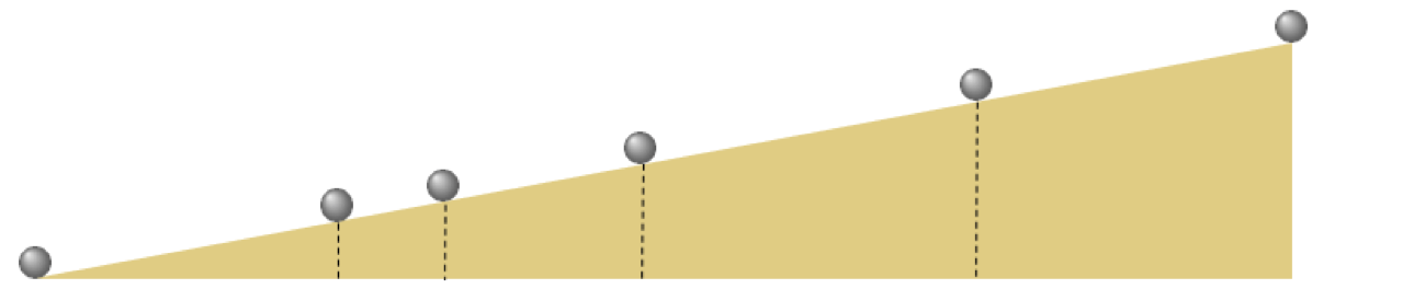
• repeatedly rolling a metal ball down a grooved $\frac{1}{2}$ meter long piece of wood set at an incline Galileo timed how long the ball took to get $\frac{1}{4}$,$\frac{1}{2}$, $\frac{2}{3}$, $\frac{3}{4}$, and all the way down the wood ramp.

• data from a modern reenactment

## This code cell will not be shown in the HTML version of this notebook
# load data
csvname = datapath + 'galileo_ramp_data.csv'
data = np.loadtxt(csvname,delimiter = ',')

# get input/output pairs
x = data[:,:-1].T
y = data[:,-1:]

# plot dataset
demo = regress_plotter.Visualizer(data)
demo.plot_data()

• and using his physical intuition Galileo - intuited a quadratic relationship

• in ML/DL jargon that for some $w_0$, $w_1$, and $w_2$ the modeling function

\begin{equation} \text{model}(x,\mathbf{w}) = w_0 + w_1x + w_2x^2 \end{equation}

• here we have two feature transformations: $f_1(x) = x$ and the quadratic term $f_2(x) = x^2$,

• build them into the same feature_transforms function

def feature_transforms(x):
    # calculate feature transform
    f = np.array([(x.flatten()**d) for d in range(1,3)])   
    return f

• minimize Least Squares cost via gradient descent using this

# plot data and fit in original and feature transformed space
ind = np.argmin(run1.cost_history)
w_best = run1.weight_history[ind]
demo.plot_fit_and_feature_space(w_best,run1.model,run1.feature_transforms,normalizer = run1.normalizer,view = [25,100])