Chapter 12: Introduction to nonlinear learning

12.2 Features, functions, and nonlinear classification

• In this Section we introduce the general framework of nonlinear classification, along with many examples.

• These examples are all low dimensional, allowing us to visually examine patterns in the data and propose appropriate nonlinearities, which we can (as we will see) very quickly inject into our linear supervised paradigm to produce nonlinear classifications.

• Just as with the previous Section by walking through these examples we flush out a number important concepts in concrete terms, coding principles, and jargon-terms in a relatively simple environment that will be omnipresent in our discussion of nonlinear learning going forward.

Activate next cell to toggle code on and off

from IPython.display import display
from IPython.display import HTML
import IPython.core.display as di # Example: di.display_html('<h3>%s:</h3>' % str, raw=True)

# This line will hide code by default when the notebook is eåxported as HTML
di.display_html('<script>jQuery(function() {if (jQuery("body.notebook_app").length == 0) { jQuery(".input_area").toggle(); jQuery(".prompt").toggle();}});</script>', raw=True)

# This line will add a button to toggle visibility of code blocks, for use with the HTML export version
di.display_html('''<button onclick="jQuery('.input_area').toggle(); jQuery('.prompt').toggle();">Toggle code</button>''', raw=True)

Toggle code

12.2.1 Modeling principles linear and nonlinear two class classification

• with two class linear classification we aim at determinig the proper parameters $\mathbf{w}$ of a linear model

\begin{equation} \text{model}\left(\mathbf{x},\mathbf{w}\right) = \mathbf{x}^T \mathbf{w} \end{equation}

that the corresponding linear decision boundary

\begin{equation} \text{model}\left(\mathbf{x},\mathbf{w}\right) = \mathbf{x}^T \mathbf{w} = 0 \end{equation}

separates the two classes as well as is possible using a linear model

• in Chapter 9 we saw several cost functions of this model, like softmax

\begin{equation} g\left(\mathbf{w}\right) = \frac{1}{P}\sum_{p=1}^{P}\text{log}\left(1 + e^{-y_p\text{model}\left(\mathbf{x}_p,\mathbf{w}\right)}\right) \end{equation}

whose minimum provides us with the weights that service our ideal as best as possible

Example 1. The perfect dataset for linear two class classification

• for linear two-classification our perfect dataset would consist of points where $\text{model}\left(\mathbf{x}_p,\mathbf{w}\right) = y_p$, i.e., points lying perfectly on the step function with linear boundary given by $\text{model}\left(\mathbf{x},\mathbf{w}\right) = 0$.

• if we examine any of the arguments in Chaper 9 used to derive logistic regression, the perceptron, or support vector machines nothing in any of these arguments relied on our use of a linear model

• a nonlinear assumption about how the classes of a dataset are distributed would lead to the same formulae

• e.g.,

\begin{equation} \text{model}\left(\mathbf{x},\mathbf{w}\right) = w_0^{\,} + {w}_{1}^{\,}\,f\left(\mathbf{x}_p\right) \end{equation}

where here $f$ is some parameterized or unparameterized nonlinear function or feature transformation

• just replace original linear model with one like this in softmax, minimize via gradient descent, etc.,

• just as with nonlinear regression we could in general just as well use a weighted sum of $B$ nonlinear functions

\begin{equation} \text{model}\left(\mathbf{x},\mathbf{w}\right) = w_0 + {w}_{1}\,f_1\left(\mathbf{x}_p\right) + {w}_{2}\,f_2\left(\mathbf{x}_p\right) + \cdots + w_B\,f_B\left(\mathbf{x}_p\right) \end{equation}

where $f_1,\,f_2,\,...\,f_B$ are nonlinear parameterized or unparameterized feature transformations and $w_0$ through $w_B$

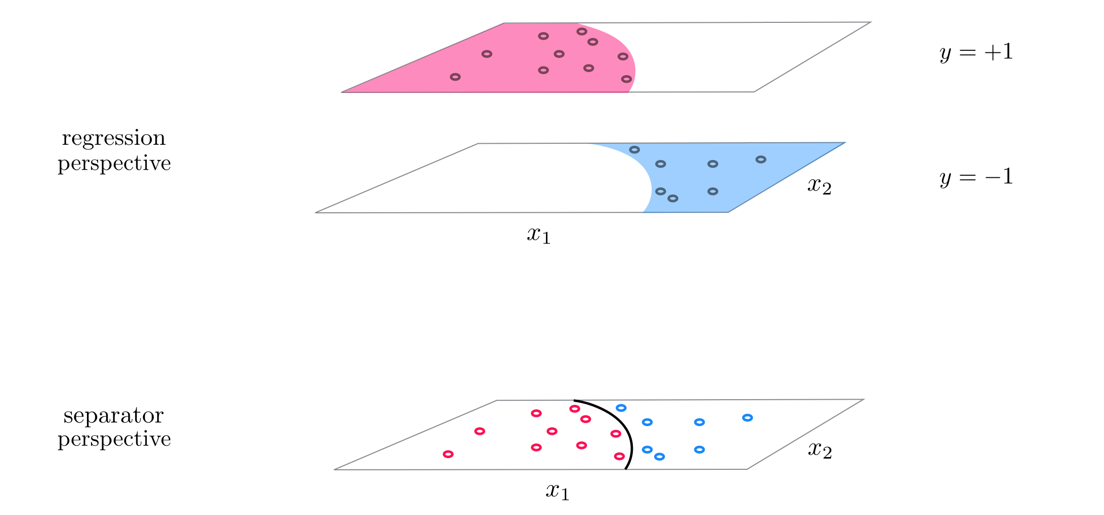
Example 2. The perfect dataset for two class nonlinear classification

• for nonlinear two-classification our perfect dataset would consist of points where the nonlinear decision boundary given by $\text{model}\left(\mathbf{x}_p,\mathbf{w}\right) = 0$ perfectly separates the data

12.2.2. Simple examples of nonlinear two class classification

• here we walk through a number of simple examples of nonlinear classification where we can determine - by eye - a proper nonlinear model

• doing this helps flush out a number of mathematical and programming concepts that are crucial going forward

• first up: its time to officially abstract our cost function(s) for two-class classification e.g., softmax

def softmax(w):
    cost = np.sum(np.log(1 + np.exp(-y*model(x,w))))
    return cost/float(len(y))

• this works regardless of the model - linear or nonlinear - so we can push it to the back

• we can also abstract our model function too, since will look essentially the same throughout all examples

• with the inclusion of general feature transformation(s) our model will always look like

# an implementation of our model employing a nonlinear feature transformation
def model(x,w):    
    # feature transformation 
    f = feature_transforms(x,w[0])
    
    # tack a 1 onto the top of each input point all at once
    o = np.ones((1,np.shape(f)[1]))
    f = np.vstack((o,f))
    
    # compute linear combination and return
    a = np.dot(f.T,w[1])
    return a

Example 4. Linear classification

## This code cell will not be shown in the HTML version of this notebook
# load data
csvname = sup_datapath + '2d_classification_data_v1.csv'
data = np.loadtxt(csvname,delimiter = ',')
x = data[:,:-1].T
y = data[:,-1:] 

# plot dataset
demo = classif_plotter.Visualizer(data)
demo.plot_data()

• employ the simple linear feature transformation

\begin{equation} f\left(x\right) = x \end{equation}

• our model is then (reduces to our typical linear model)

\begin{equation} \text{model}\left(x,\mathbf{w}_{\!}\right) = w_0 + w_{1\,}f\left(x\right). \end{equation}

# the trivial linear feature transformation
def feature_transforms(x):      
    return x

• tune via gradient descent

## This code cell will not be shown in the HTML version of this notebook
# pluck out best weights - those that provided lowest cost, 
# and plot resulting fit
ind = np.argmin(run.cost_history)
w_best = run.weight_history[ind]
demo.plot_fit(w_best,run.model,normalizer = run.normalizer);

Example 4. A one dimensional example of nonlinear classification

## This code cell will not be shown in the HTML version of this notebook
# load data
csvname = datapath + 'signed_projectile.csv'
data = np.loadtxt(csvname,delimiter = ',')
x = data[:,:-1].T
y = data[:,-1:] 

# plot dataset
demo = classif_plotter.Visualizer(data)
demo.plot_data()

• what sort of simple function crosses the horizontal axis twice?

</figure> </p>

• here we have two unparameterized feature transformations: the identity $f_1(x) = x$ and the quadratic term $f_2(x) = x^2$

• our model is then

\begin{equation} \text{model}(x,\mathbf{w}) = w_0 + w_1\,f_1(x) + w_2\,f_2(x) \end{equation}

• Python implementation

# our quadratic feature transformation
def feature_transforms(x):
    # calculate feature transform
    f = np.array([(x.flatten()**d) for d in range(1,3)])   
    return f

• tune via gradient descent

• akin to regression, what is a nonlinear model in the original space is linear in the feature transformed space

## This code cell will not be shown in the HTML version of this notebook
# plot data and fit in original and feature transformed space
ind = np.argmin(run.cost_history)
w_best = run.weight_history[ind]
demo.plot_fit_and_feature_space(w_best,run.model,run.feature_transforms,normalizer = run.normalizer,view = [25,35])

Example 5. Finding an elliptical boundary separating two classes

## This code cell will not be shown in the HTML version of this notebook
# create instance of linear regression demo, used below and in the next examples
demo = nonlib.nonlinear_classification_visualizer.Visualizer(datapath + 'ellipse_2class_data.csv')
x = demo.x.T
y = demo.y[:,np.newaxis]

# an implementation of the least squares cost function for linear regression for N = 2 input dimension datasets
demo.plot_data();

• looks like some sort of elliptical decision boundary centered at the origin might do a fine job of classification

• so a model of the form

\begin{equation} \text{model}(\mathbf{x},\mathbf{w}) = w_0^{\,} + w_1^{\,} x_1^2 + w_2^{\,}x_2^2. \end{equation}

• here we have used two feature transformations $f_1(\mathbf{x})=x_1^2$ and $f_2(\mathbf{x}) = x_2^2$

• in Python our feature_transforms function

# a elliptical feature transformation
def feature_transforms(x):
    # calculate feature transform
    f = x**2  
    return f

• now we minimize the softmax above via gradient descent.

## This code cell will not be shown in the HTML version of this notebook
# illustrate results
ind = np.argmin(run.cost_history)
w_best = run.weight_history[ind]
demo.static_N2_img(w_best,run,view1 = [20,45],view2 = [20,30])

Example 6. Using a parameterized sinusoid to classify stripes of data

## This code cell will not be shown in the HTML version of this notebook
# create instance of linear regression demo, used below and in the next examples
demo = nonlib.nonlinear_classification_visualizer.Visualizer(datapath + 'diagonal_stripes.csv')

x = demo.x.T
y = demo.y[:,np.newaxis]

# an implementation of the least squares cost function for linear regression for N = 2 input dimension datasets
demo.plot_data();

• a completely parameterized sinusoid of two inputs

\begin{equation} f\left(\mathbf{x}\right) = \text{sin}\left(w_0 + w_1x_1 + w_2x_2\right). \end{equation}

• our model a linear combination of this nonlinear feature transformation as

\begin{equation} \text{model}\left(\mathbf{x},\mathbf{w}_{\!}\right) = w_3 + w_{4\,}f\left(\mathbf{x},\mathbf{w}\right). \end{equation}

- in `Python` our `feature_transforms` function

# our nonlinearity, known as a feature transformation
def feature_transforms(x,w):
    # tack a 1 onto the top of each input point all at once
    o = np.ones((1,np.shape(x)[1]))
    x = np.vstack((o,x))
        
    # calculate feature transform
    f = np.sin(np.dot((x).T,w)).T
    return f

• tune via gradient descent using softmax cost

## This code cell will not be shown in the HTML version of this notebook
# illustrate results
ind = np.argmin(run.cost_history)
w_best = run.weight_history[ind]
demo.static_N2_simple(w_best,run,view = [30,155])

12.2.3 Modeling principles linear and nonlinear multiclass classification

• can inject nonlinearity into our mulitclass classification in the same way we have done for two-class scenario

• regardless of framework we always aim to learn $C$ classifiers, do the same thing we have done above for each

• simply inject nonlinear feature transforms in the same way we have seen done above

• some small technical differences, see notes for details

12.2.4 Simple examples of nonlinear multiclass classification

Example 7. Nonlinear One-versus-All multiclass classification

## This code cell will not be shown in the HTML version of this notebook
# create instance of linear regression demo, used below and in the next examples
demo = nonlib.nonlinear_classification_visualizer.Visualizer(datapath + '3_layercake_data.csv')
x = demo.x.T
y = demo.y[:,np.newaxis]

# an implementation of the least squares cost function for linear regression for N = 2 input dimension datasets
demo.plot_data();

• looks like the classes of this dataset can be cleanly separated via elliptical boundaries, but the distribution of each class is not centered at the origin

• to capture this behavior we will use a full degree 2 polynomial expansion of the input

• terms from a general degree $D$ polynomial always take the form

\begin{equation} f\left(\mathbf{x}\right) = x_1^ix_2^j \end{equation}

where $i + j \leq D$.

• to employ all of them for $D = 2$ means using the following nonlinear model

\begin{equation} \text{model}\left(\mathbf{x},\mathbf{w}\right) = w_0 + w_1x_1 + w_2x_2 + w_3x_1x_2 + w_4x_1^2 + w_5x_2^2 \end{equation}

In Python we can implement this in a feature_transforms as follows.

# a elliptical feature transformation
def feature_transforms(x):
    # calculate feature transform
    f = []
    for i in range(0,D):
        for j in range(0,D-i):
            if i > 0 or j > 0:
                term = (x[0,:]**i)*((x[1,:])**j)
                f.append(term)
    return np.array(f)

• Use One-versus-All framework, softmax cost and gradient descent for each classifier

## This code cell will not be shown in the HTML version of this notebook
# draw resulting nonlinear boundaries for each classification problem, as well as the
# entire multiclass boundary
run = nonlib.basic_runner.Setup(x,y,feature_transforms,'multiclass_counter',normalize = 'standard')
w_best = combined_weights[-1]
demo.show_individual_classifiers(run,w_best)

Example 8. Nonlinear multiclass softmax classification

• repeat previous experiment, but with multiclass softmax cost function

## This code cell will not be shown in the HTML version of this notebook
# plot result of nonlinear multiclass classification
w_best = combined_weights[-1]
demo.multiclass_plot(run,w_best)