12.3 Features, functions, and nonlinear unsupervised learning
Press the button 'Toggle code' below to toggle code on and off for entire this presentation.
from IPython.display import display
from IPython.display import HTML
import IPython.core.display as di # Example: di.display_html('<h3>%s:</h3>' % str, raw=True)

# This line will hide code by default when the notebook is eåxported as HTML
di.display_html('<script>jQuery(function() {if (jQuery("body.notebook_app").length == 0) { jQuery(".input_area").toggle(); jQuery(".prompt").toggle();}});</script>', raw=True)

# This line will add a button to toggle visibility of code blocks, for use with the HTML export version
di.display_html('''<button onclick="jQuery('.input_area').toggle(); jQuery('.prompt').toggle();">Toggle code</button>''', raw=True)
12.3.1 Modeling principles of the linear and nonlinear autoencoder
Recall the autoencoder cost function
\begin{equation} g\left(\mathbf{C}\right) = \frac{1}{P}\sum_{p = 1}^P \left \Vert \mathbf{C}_{\,}^{\,}\mathbf{C}_{\,}^T\mathbf{x}_p - \mathbf{x}_p \right\Vert_2^2 \end{equation}Note we can break up the term $\mathbf{C}\mathbf{C}^T\mathbf{x}_p$ into an explicit encoding and decoding step. We have our encoder function $f_{\text{e}}$
and decoder function $f_{\text{d}}$
Their composition evaluated at $\mathbf{x}_p$ is then given as
\begin{equation} f_{\text{d}}\left(\,f_{\text{e}}\left(\mathbf{x}_p\right)\right) = \mathbf{C}_{\,}^{\,}\mathbf{C}_{\,}^T\mathbf{x}_p \end{equation}Note: for simplicity, we have left off the encoder and decoder's dependency on internal parameters. To be more accurate we should write $f_{\text{d}}\left(\mathbf{v},\mathbf{C}\right)$ and $f_{\text{e}}\left(\mathbf{x},\mathbf{C}\right)$.
This allows us to write the autoencoder cost function more generally as
\begin{equation} g\left(\mathbf{C}\right) = \frac{1}{P}\sum_{p = 1}^P \left \Vert \,f_{\text{d}}\left(\,f_{\text{e}}\left(\mathbf{x}_p\right)\right) - \mathbf{x}_p \right\Vert_2^2 \end{equation}Python implementation:
We can process the entire dataset $\mathbf{X}$ in one operation (which is more efficient in Python than explicitly looping over the points).
# a linear encoder function
def encoder(X,C):
    return np.dot(C.T,X)

# a linear decoder function
def decoder(V,C):
    return np.dot(C,V)
We can wrap up the encoder and decoder using our typical model function, producing $f_{\text{d}}\left(\,f_{\text{e}}\left(\mathbf{x}_p\right)\right)$.
# a model function wrapping up our linear encoding/decoding schemes
def model(X,C):
    # encode the input
    V = encoder(X,C)

    # decode the encoding
    a = decoder(V,C)
    return a
To tune these parameters properly we can then minimize the autoencoder function below using e.g., gradient descent.
# an implementation of the least squares cost function for linear regression
def autoencoder(C):
    cost = np.sum((model(X,C) - X)**2)
    return cost/float(X.shape[1])
Example 1. Linear PCA using the autoencoder
# load in a dataset to learn a PCA basis for via the autoencoder
X = np.loadtxt(datapath + '2d_span_data_centered.csv',delimiter=',')

# scatter dataset
fig = plt.figure(figsize = (9,4))
gs = gridspec.GridSpec(1,1)
ax = plt.subplot(gs[0],aspect = 'equal');
ax.set_xlabel(r'$x_1$',fontsize = 15);ax.set_ylabel(r'$x_2$',fontsize = 15,rotation = 0);
ax.scatter(X[0,:],X[1,:],c = 'k',s = 60,linewidth = 0.75,edgecolor = 'w');

Using gradient descent we then minimize the autoencoder cost, finding the best one dimensional subspace for this two-dimensional dataset.
# tune the autoencoder via gradient descent
g = autoencoder; alpha_choice = 10**(-2); max_its = 1000; C = 0.1*np.random.randn(2,1);
weight_history,cost_history = optimizers.gradient_descent(g,alpha_choice,max_its,C)
# plot results
unlib.autoencoder_demos.show_encode_decode(X,cost_history,weight_history,show_pc = True,scale = 150,encode_label = r'$\mathbf{c}$',projmap = True)


Nonlinear autoencoders?
- Just like we extended linear regression/classification to nonlinear regression/classification, we can extend the autoencoder framework so that it uses nonlinear encoder and decoder instead of linear ones.
- To make this extension we can introduce any two parameterized nonlinear functions: one for
encoding$\,\,f_{\text{e}}\left(\mathbf{x}\right)$ and one fordecoding$ f_{\text{d}}\left(\mathbf{v}\right)$ so that again we have
We can still use the same autoencoder cost function
\begin{equation} g\left(\mathbf{w}\right) = \frac{1}{P}\sum_{p = 1}^P \left \Vert \,f_{\text{d}}\left(\,f_{\text{e}}\left(\mathbf{x}_p\right)\right) - \mathbf{x}_p \right\Vert_2^2 \end{equation}where $\mathbf{w}$ denotes the entire set of parameters of both the encoder $f_{\text{e}}$ and decoder $f_\text{d}$.
12.1.3 Introductory examples of nonlinear PCA via the autoencoder
Python implementation:
- We can virtually re-use most of the code framework we employed in the linear case.
- We only need to slightly modify the
modelfunction to take in a generally larger set of parameters - since each of our encoding/decoding functions can in general have unique sets of parameters.
# a general model wrapping up our encoder/decoder
def model(X,w):
    # encode the input
    v = encoder(X,w[0])

    # decode the encoding
    a = decoder(v,w[1])
    return a
Example 2. Finding a circular subspace via the autoencoder
# import data
X = np.loadtxt(datapath + 'circle_data.csv',delimiter=',')

# scatter dataset
fig = plt.figure(figsize = (9,4))
gs = gridspec.GridSpec(1,1)
ax = plt.subplot(gs[0],aspect = 'equal');
ax.set_xlabel(r'$x_1$',fontsize = 15);ax.set_ylabel(r'$x_2$',fontsize = 15,rotation = 0);
ax.scatter(X[0,:],X[1,:],c = 'k',s = 60,linewidth = 0.75,edgecolor = 'w')
plt.show()

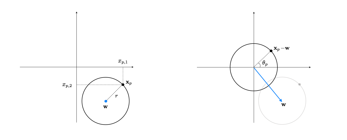
Encoder design:
- We subtract off $\mathbf{w}$ from any $\mathbf{x}_p$ in the dataset. This centers the circle around the origin.
- Using the arctan function we can then find the angle $\theta_p$ - this is the encoded version of $\mathbf{x}_p$.
def my_arctan(x1,x2):
    v = x2/x1
    if x1 > 0:
        return np.arctan(v)
    elif x1 < 0 and x2 >= 0:
        return np.arctan(v) + np.pi
    elif x1 < 0 and x2 < 0:
        return np.arctan(v) - np.pi
    elif x1==0 and x2 > 0:
        return np.pi*0.5
    elif x1==0 and x2 < 0:
        return -np.pi*0.5

def encoder(x,w):
    a = x - w
    b = []
    for i in range(a.shape[1]):
        b.append(my_arctan(a[0][i],a[1][i]))
    b = np.array(b)[np.newaxis,:]
    return b
Decoder design:
beginning with $\theta_p$ as the encoded version of $\mathbf{x}_p$ we form the vector $\left[\begin{array}{c} r_1\,\text{cos}(\theta_p)\\ r_2\,\text{sin}(\theta_p) \end{array}\right]$ where we use potentially different parameters $r_1$ and $r_2$, in case the original data wasn't a perfect circle.
The decoded version of $\theta_p$ is then given by $\left[\begin{array}{c} r_1\,\text{cos}(\theta_p)\\ r_2\,\text{sin}(\theta_p) \end{array}\right] + \mathbf{w}$. One can reuse the same $\mathbf{w}$ learned through encoding or learn it altogther independent of the encoder. The take the latter approach.
def decoder(v,w):
    a = w[:,0][:,np.newaxis]*np.vstack((np.cos(v),np.sin(v))) + w[:,1][:,np.newaxis]
    return a
Using gradient descent we can now minimize the autoencoder cost, finding the optimal encoder/decoder parameters for this dataset.
scale = 0.1
w = [scale*np.random.randn(2,1),scale*np.random.randn(2,2)];

# tune pca least squares cost
g = autoencoder;

# tune pca least squares cost
alpha_choice = 10**(-1); max_its = 100;
weight_history,cost_history = optimizers.gradient_descent(g,alpha_choice,max_its,w)

# plot the cost function history for a given run
static_plotter.plot_cost_histories([cost_history],start = 0,points = False,labels = [r'$\alpha = 1$'])

# plot results
unlib.autoencoder_demos.show_encode_decode(X,cost_history,weight_history,encoder=encoder,decoder=decoder,show_pc = False,scale = 55,encode_label = r'$\mathbf{c}$',projmap = True)

