13.1 Multi-layer perceptrons (MLPs)

Press the button 'Toggle code' below to toggle code on and off for entire this presentation.

from IPython.display import display
from IPython.display import HTML
import IPython.core.display as di # Example: di.display_html('<h3>%s:</h3>' % str, raw=True)

# This line will hide code by default when the notebook is eåxported as HTML
di.display_html('<script>jQuery(function() {if (jQuery("body.notebook_app").length == 0) { jQuery(".input_area").toggle(); jQuery(".prompt").toggle();}});</script>', raw=True)

# This line will add a button to toggle visibility of code blocks, for use with the HTML export version
di.display_html('''<button onclick="jQuery('.input_area').toggle(); jQuery('.prompt').toggle();">Toggle code</button>''', raw=True)

Toggle code

• At the heart of nonlinear learning is the following simple yet powerful idea: nonlinear curves of arbitrary shape can be expressed/approximated via a linear combination of simpler nonlinear functions of the input data that are organized in a way to form a basis.

• With neural networks each of these basis functions is also parameterized with a number of weights to be tuned using data.

• Here we discuss in detail how to form neural network basis functions starting with the simplest of them: a single-layer function.

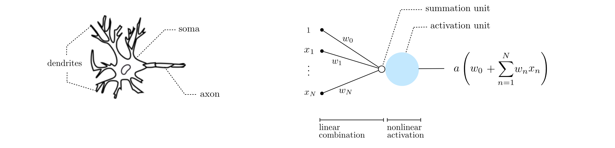
13.1.1 Single-layer basis functions

Recursive rescipe for single layer basis functions

I. Take a linear combination of the input (plus a bias): $w_{0}+{\sum_{n=1}^{N}}{w_{n}\,x_n}$

II. Pass the result through a nonlinear function: $a\left(w_{0}+{\sum_{n=1}^{N}}{w_{n}\,x_n}\right)$

Note: step 1 makes the resulting basis function parameterized while step 2 makes it nonlinear.

Example 1. The shape of single-layer functions with $\text{tanh}$ activation

Four instances of a single-layer basis function using $\text{tanh}$ as nonlinear activation function and randomly set weights:

\begin{equation} f^{(1)}(x) = \text{tanh}\left(w_0 + w_1x\right) \end{equation}

# import Draw_Bases class for visualizing various basis element types
demo = nonlib.DrawBases.Visualizer()

# plot the first 4 elements of a single layer basis
demo.show_1d_net(num_layers = 1, activation = 'tanh')

Example 2. The shape of single-layer functions with ReLU activation

\begin{equation} f^{(1)}(x) = \text{max}\left(0,w_0 + w_1x\right) \end{equation}

# import Draw_Bases class for visualizing various basis element types
demo = nonlib.DrawBases.Visualizer()

# plot the first 4 elements of a single hidden layer basis
demo.show_1d_net(num_layers = 1, activation = 'relu')

Graphical representation of single layer basis functions

Figure 1: (left) A typical biological neuron. (right) An artificial neuron (perceptron). A perceptron is a simplistic mathematical model for the biological neuron consisting of: (i) weighted edges that represent the individual multiplications (of $1$ by $w_{0}$, $x_1$ by $w_{1}$, etc.), (ii) a summation unit shown as a small hollow circle representing the sum $w_0+w_{1}\, x_1+\cdots+w_{N}\, x_N$, and (iii) an activation unit shown as a larger blue circle representing the sum evaluated by the nonlinear activation function $a$.

Algebraic representation of single layer basis functions

\begin{equation} f\left(x_1,x_2,\ldots,x_N\right)=a\left(w_{0}+\underset{n=1}{\overset{N}{\sum}}{w_{n}\,x_n}\right) \end{equation}

13.1.2 Two-layer basis functions

Recursive rescipe for three layer basis functions

I. Take a linear combination of $U_1$ single-layer functions (plus a bias): $w_{0}+{\sum_{j=1}^{U_1}}{w_{j}\,f^{(1)}_j}$

II. Pass the result through the nonlinear activation function: $a\left(w_{0}+{\sum_{j=1}^{U_1}}{w_{j}\,f^{(1)}_j}\right)$

Example 3. The shape of two-layer functions with $\text{tanh}$ activation

Four instances of a two-layer basis function using $\text{tanh}$ as activation, with randomly set weights, each taking the form

\begin{equation} f^{(2)}(x) = \text{tanh}\left(w_2 + w_3\,f^{(1)}(x)\right) \end{equation}

where

\begin{equation} f^{(1)}(x) = \text{tanh}\left(w_0 + w_1x\right) \end{equation}

# import Draw_Bases class for visualizing various basis element types
demo = nonlib.DrawBases.Visualizer()

# plot the first 4 elements of the polynomial basis
demo.show_1d_net(num_layers = 2, activation = 'tanh')

Graphical representation of two layer basis functions

Figure 2: Graphical representation of a two-layer neural network basis function. (left) A two-layer element is constructed by cascading a series of $U_1$ perceptron units, and connecting their outputs to another perceptron unit in the second layer. (right) A more compact representation of the two-layer element on the left. See the text for more description.

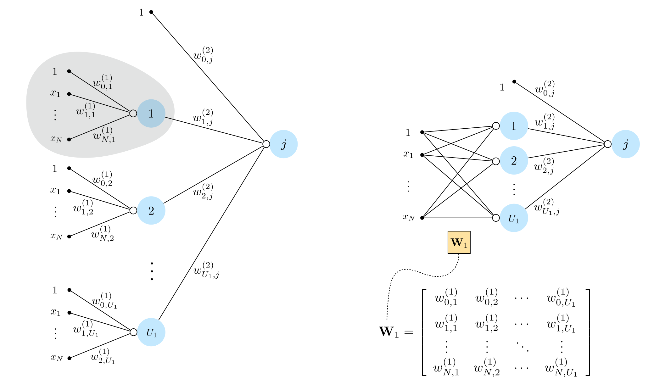
Algebraic representation of two layer basis functions

\begin{equation} f_j^{\left(2\right)}\left(x_1,x_2,\ldots,x_N\right)=a\left(w^{\left(2\right)}_{0,j}+\underset{i=1}{\overset{U_1}{\sum}}{w^{\left(2\right)}_{i,j}}\,a\left(w^{\left(1\right)}_{0,i}+\underset{n=1}{\overset{N}{\sum}}{w^{\left(1\right)}_{n,i}\,x_n}\right)\right) \end{equation}

13.1.3 Three-layer basis functions

Recursive rescipe for three layer basis functions

I. Take a linear combination of the $U_2$ two-layer functions (plus a bias): $w_{0}+{\sum_{j=1}^{U_2}}{w_{j}\,f^{(2)}_j}$

II. Pass the result through the activation function: $a\left(w_{0}+{\sum_{j=1}^{U_2}}{w_{j}\,f^{(2)}_j}\right)$

Example 4. The shape of three-layer functions with $\text{tanh}$ activation

# import Draw_Bases class for visualizing various basis element types
demo = nonlib.DrawBases.Visualizer()

# plot the first 4 elements of the polynomial basis
demo.show_1d_net(num_layers = 3, activation = 'tanh')

Graphical representation of three layer basis functions

Figure 3: Graphical representation of a three-layer basis function. (left) A three-layer element is constructed by cascading a series of $U_2$ 2-layer elements (the first of which is encompassed in a gray bubble), and connecting their outputs to another perceptron unit in the third layer. (right) An equivalent but more condensed representation of the three-layer element on the left. See the text for more description.

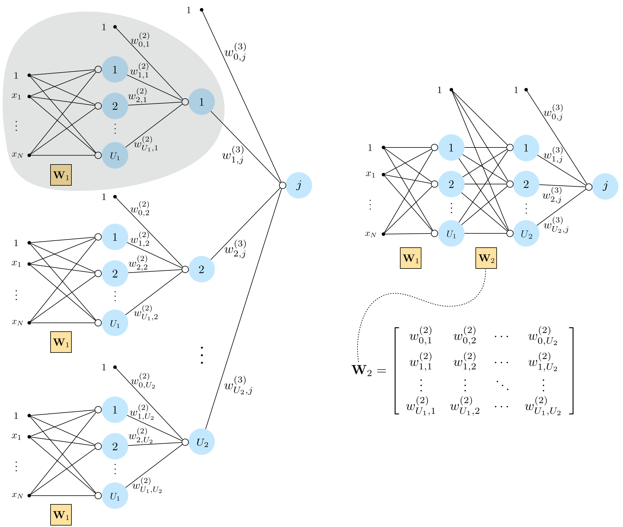
Algebraic representation of three layer basis functions

\begin{equation} f_j^{\left(3\right)}\left(x_1,x_2,\ldots,x_N\right)=a_{\,}\left(w^{\left(3\right)}_{0,j}+\underset{i=1}{\overset{U_2}{\sum}}{w^{\left(3\right)}_{i,j}}\,a_{\,}\left(w^{\left(2\right)}_{0,i}+\underset{k=1}{\overset{U_1}{\sum}}{w^{\left(2\right)}_{k,i}}\,a_{\,}\left(w^{\left(1\right)}_{0,k}+\underset{n=1}{\overset{N}{\sum}}w^{\left(1\right)}_{n,k}\,x_n\right)\right)\right) \end{equation}

13.1.4 General multilayer basis functions

Recursive recipe for $L$-layer basis functions

I. Take a linear combination of the $(L-1)$-layer basis functions (plus a bias): $w_{0}+{\sum_{j=1}^{U_{L-1}}}{w_{j}\,f^{(L-1)}_j}$

II. Pass the result through the activation function: $a\left(w_{0}+{\sum_{j=1}^{U_{L-1}}}{w_{j}\,f^{(L-1)}_j}\right)$

Graphical representation of multilayer basis functions

Figure 4: (top) Graphical representation of an $L$-layer neural network basis function. The $k^{th}$ layer weights are stored in the matrix $\mathbf{W}_k$ as defined in (5), for all $k=1,\ldots, L-1$. (bottom) Using equations (6-8) we can draw the computational graph of an $L$-layer basis function as a convenient replacement for the graphical representation shown in the top panel. As is our convention with computational graphs, we represent scalar, vector, and matrix variables with circles, diamonds, and squares, respectively.

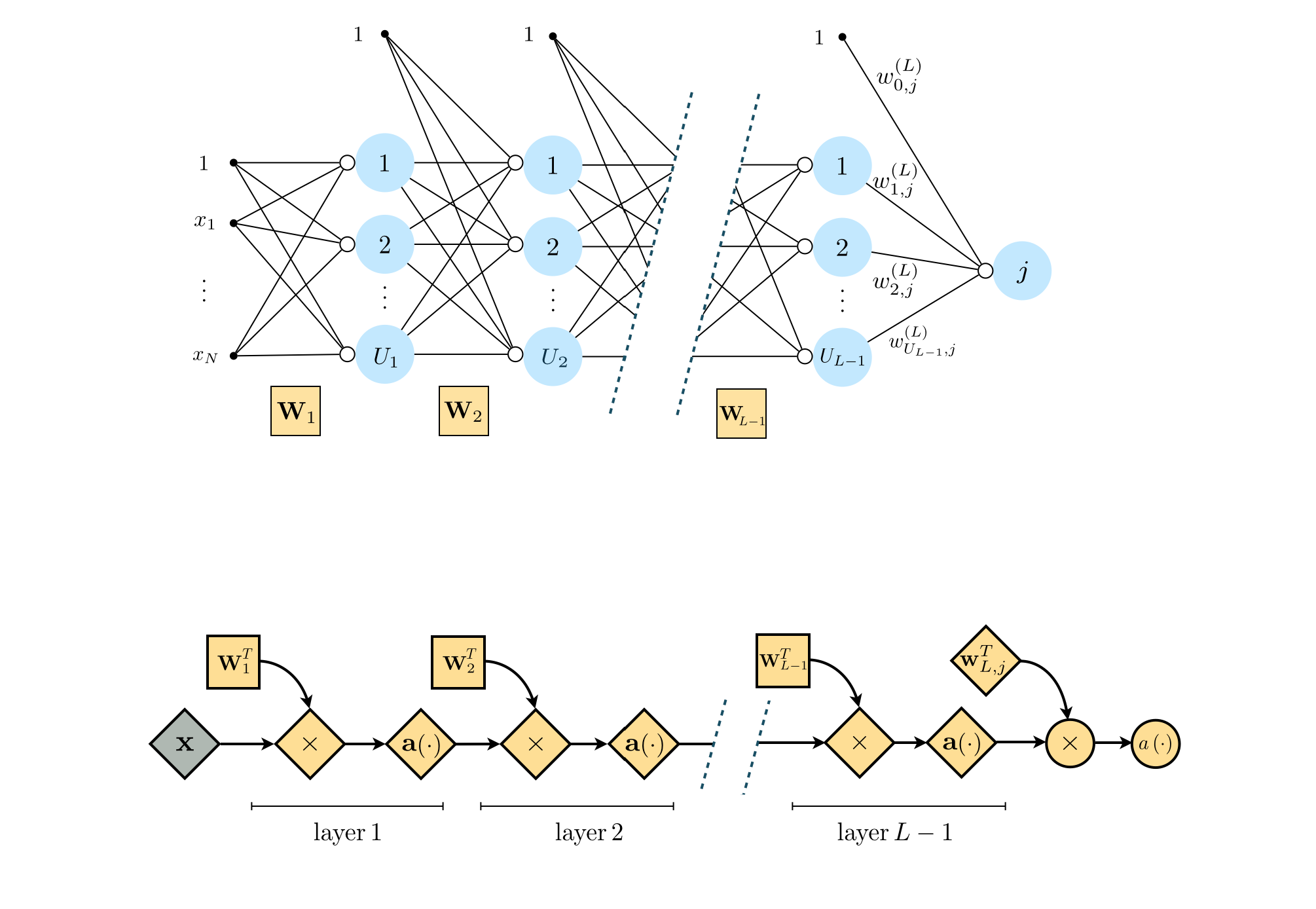
Algebraic representation of multilayer basis functions

\begin{equation} f_j^{\left(L\right)}\left(\mathbf{x}\right)=a\left(\mathbf{w}_{L,j}^T\,\mathbf{a}\,\left(\mathbf{W}_{L-1}^T\,\cdots\,\mathbf{a}\,\left(\mathbf{W}_{2}^T\,\mathbf{a}\left(\mathbf{W}_{1}^T\,\mathbf{x}\right)\right)\right)\right) \end{equation}

13.1.5 Implementing multilayer perceptrons from scratch

The feature_transforms module below returns $\mathbf{f}$ as a function of $\mathbf{x}$: the input data, and $\mathbf{w}$: a tensor of weights $\mathbf{W}_1$ through $\mathbf{W}_L$.

# choose a nonlinear activation function 
def activation(t):
    nonlinearity = np.tanh(t)
    return nonlinearity

# fully evaluate our network features using the tensor of weights in w
def feature_transforms(a, w):    
    # loop through each layer matrix
    for W in w:
        #  pad with ones (to compactly take care of bias) for next layer computation        
        o = np.ones((1,np.shape(a)[1]))
        a = np.vstack((o,a))
        
        # compute inner product with current layer weights
        a = np.dot(a.T, W).T
    
        # output of layer activation
        a = activation(a)
    return a

The initialize_network_weights module creates initial weights for a feedforward network, and also provides a simple interface for generating feedforward architectures with arbitrary numbers of layers.

\begin{equation} \text{layer_sizes} = \begin{bmatrix} N = \text{dimension of input }\mathbf{x} \,\,\,\,\,\,\,\,\,\,\,\,\,\,\,\,\,\,\,\,\,\,\,\,\,\,\, \\ U_1 = \text{number of desired units in layer 1} \\ U_2 = \text{number of desired units in layer 2} \\ \vdots \\ U_L = \text{number of desired units in layer L} \\ M = \text{dimension of output } y \,\,\,\,\,\,\,\,\,\,\,\,\,\,\,\,\,\,\,\,\,\,\,\,\, \end{bmatrix} \end{equation}

# create initial weights for arbitrary feedforward network
def initialize_network_weights(layer_sizes, scale):
    # container for entire weight tensor
    weights = []
    
    # loop over desired layer sizes and create appropriately sized initial 
    # weight matrix for each layer
    for k in range(len(layer_sizes)-1):
        # get layer sizes for current weight matrix
        U_k = layer_sizes[k]
        U_k_plus_1 = layer_sizes[k+1]

        # make weight matrix
        weight = scale*np.random.randn(U_k+1,U_k_plus_1)
        weights.append(weight)

    # re-express weights so that w_init[0] = omega_inner contains all 
    # internal weight matrices, and w_init = w contains weights of 
    # final linear combination in predict function
    w_init = [weights[:-1],weights[-1]]
    
    return w_init

Example 5. Nonlinear regression using MLP

# load data
csvname = datapath + 'noisy_sin_sample.csv'
data = np.loadtxt(csvname,delimiter = ',')
x = data[:,:-1].T
y = data[:,-1:] 

# plot dataset
demo = regress_plotter.Visualizer(data)
demo.plot_data()

We will use a 4 layer network with 10 units in each layer.

# An example 4 hidden layer network, with 10 units in each layer
N = 1
M = 1
U_1 = 10
U_2 = 10
U_3 = 10
U_4 = 10

# the list defines our network architecture
layer_sizes = [N, U_1,U_2,U_3,U_4,M]

# generate initial weights for our network
w = initialize_network_weights(layer_sizes, scale = 0.5)

# run
alpha_choice = 10**(-1); max_its = 1000;
run = nonlib.basic_runner.Setup(x,y,feature_transforms,'least_squares',normalize = 'standard')
run.fit(w=w,alpha_choice = alpha_choice,max_its=max_its)

# plot the cost function history for a given run
static_plotter.plot_cost_histories([run.cost_history],start = 0,points = False,labels = ['run 1'])

# pluck out best weights - those that provided lowest cost, 
# and plot resulting fit
ind = np.argmin(run.cost_history)
w_best = run.weight_history[ind]
demo.plot_fit(w_best,run.model,normalizer = run.normalizer);

Example 6. Nonlinear two-class classification example using MLP

# create instance of linear regression demo, used below and in the next examples
demo = nonlib.nonlinear_classification_visualizer.Visualizer(datapath + '2_eggs.csv')
x = demo.x.T
y = demo.y[:,np.newaxis]

# an implementation of the least squares cost function for linear regression for N = 2 input dimension datasets
demo.plot_data();

Again, 4 hidden layers with 10 units in each layer.

# An example 4 hidden layer network, with 10 units in each layer
N = 2
M = 1
U_1 = 10
U_2 = 10
U_3 = 10

# the list defines our network architecture
layer_sizes = [N, U_1,U_2,U_3,M]

# generate initial weights for our network
w = initialize_network_weights(layer_sizes, scale = 0.5)

# parameters for our two runs of gradient descent
max_its = 1000; alpha_choice = 10**(0)

# run on normalized data
run = nonlib.basic_runner.Setup(x,y,feature_transforms,'softmax',normalize = 'standard')
run.fit(w=w,alpha_choice = alpha_choice,max_its = max_its)

# plot the cost function history for a given run
static_plotter.plot_cost_histories([run.cost_history],start = 0,points = False,labels = ['run 1'])

# illustrate results
ind = np.argmin(run.cost_history)
w_best = run.weight_history[ind]
demo.static_N2_simple(w_best,run,view = [30,155])