13.4 The momentum trick

Press the button 'Toggle code' below to toggle code on and off for entire this presentation.

from IPython.display import display
from IPython.display import HTML
import IPython.core.display as di # Example: di.display_html('<h3>%s:</h3>' % str, raw=True)

# This line will hide code by default when the notebook is eåxported as HTML
di.display_html('<script>jQuery(function() {if (jQuery("body.notebook_app").length == 0) { jQuery(".input_area").toggle(); jQuery(".prompt").toggle();}});</script>', raw=True)

# This line will add a button to toggle visibility of code blocks, for use with the HTML export version
di.display_html('''<button onclick="jQuery('.input_area').toggle(); jQuery('.prompt').toggle();">Toggle code</button>''', raw=True)

Toggle code

When the minimum lies in a long narrow valley, the negative gradient at $\mathbf{w}^{k}$, being perpendicular to the contour line at that point, points far away from the optimal direction.

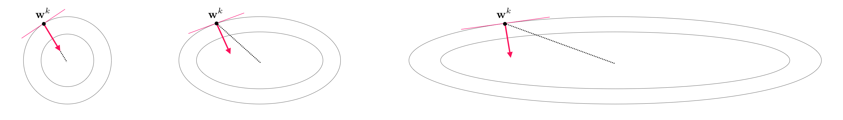
The progress of gradient descent is significantly slowed down in this case as gradient descent steps tend to zig-zag towards a solution.

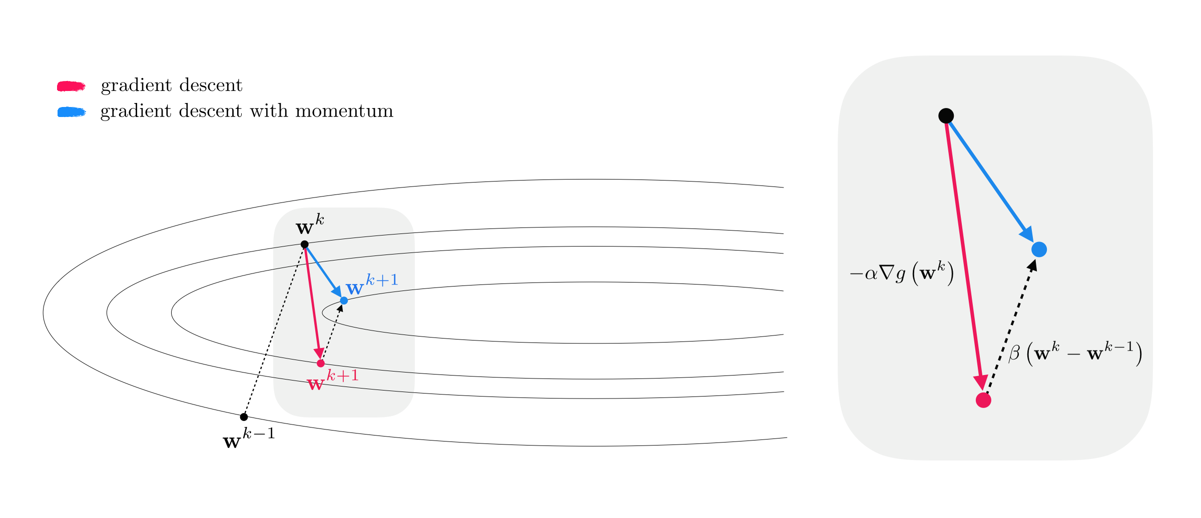
This problem motivates the concept of an old and simple heuristic known as the momentum term.

The momentum term is a simple weighted difference of the subsequent $k^{th}$ and $(k−1)^{th}$ gradient steps, i.e., $\beta \left(\mathbf{w}^k - \mathbf{w}^{k-1}\right)$ for some $\beta >0$.

Alternative derivation:

\begin{equation} \mathbf{w}^{k+1} = \mathbf{w}^k - \alpha \nabla g\left(\mathbf{w}^k\right) + \beta \left(\mathbf{w}^{k} - \mathbf{w}^{k-1}\right) \end{equation}

I. Subtract $\mathbf{w}_k$ from both sides and divide them by $-\alpha$

\begin{equation} \frac{1}{-\alpha}\left(\mathbf{w}^{k+1}-\mathbf{w}^k\right) = \nabla g\left(\mathbf{w}^k\right) - \frac{\beta}{\alpha} \left(\mathbf{w}^{k} - \mathbf{w}^{k-1}\right) \end{equation}

II. Denote the left hand side by a new variable $\mathbf{z}^{k+1} = \frac{1}{-\alpha}\left(\mathbf{w}^{k+1}-\mathbf{w}^k\right)$ to write the above as

\begin{equation} \mathbf{z}^{k+1} = \nabla g\left(\mathbf{w}^k\right) +\beta\, \mathbf{z}^{k} \end{equation}

Alternative derivation:

\begin{equation} \begin{array} \ \mathbf{z}^{k+1} = \beta\,\mathbf{z}^{k} + \nabla g\left(\mathbf{w}^k\right) \\ \mathbf{w}^{k+1} = \mathbf{w}^{k} - \alpha \, \mathbf{z}^{k+1} \end{array} \end{equation}

def gradient_descent(g,w,alpha,max_its,beta,version):    
    # flatten the input function, create gradient based on flat function
    g_flat, unflatten, w = flatten_func(g, w)
    grad = compute_grad(g_flat)

    # record history
    w_hist = []
    w_hist.append(unflatten(w))

    # start gradient descent loop
    z = np.zeros((np.shape(w)))      # momentum term
    
    # over the line
    for k in range(max_its):   
        # plug in value into func and derivative
        grad_eval = grad(w)
        grad_eval.shape = np.shape(w)

        ### normalized or unnormalized descent step? ###
        if version == 'normalized':
            grad_norm = np.linalg.norm(grad_eval)
            if grad_norm == 0:
                grad_norm += 10**-6*np.sign(2*np.random.rand(1) - 1)
            grad_eval /= grad_norm
            
        # take descent step with momentum
        z = beta*z + grad_eval
        w = w - alpha*z

        # record weight update
        w_hist.append(unflatten(w))

    return w_hist

Example 1. Using momentum to speed up the minimization of simple quadratic functions

\begin{equation} g(\mathbf{w}) = a + \mathbf{b}^T\mathbf{w} + \mathbf{w}^T\mathbf{C}\mathbf{w} \end{equation}

$a = 0$, $\mathbf{b} = \begin{bmatrix} 1 \\ 1 \end{bmatrix}$, $\mathbf{C} = \begin{bmatrix} 1\,\,0 \\ 0 \,\, 12\end{bmatrix}$

$\beta = 0.3$

# visualize
demo = nonlib.contour_run_comparison.Visualizer()
demo.show_paths(g, weight_history_1,weight_history_4,num_contours = 20)

A longer and narrower valley requires a larger $\beta$ (here $\beta=0.7$)

# visualize
demo = nonlib.contour_run_comparison.Visualizer()
demo.show_paths(g, weight_history_1,weight_history_2,num_contours = 20)

Example 2. Using momentum to speed up the minimization of linear two-class classification

Non-convex functions can too have problematic long narrow valleys (in this case the logistic Least Squares cost).

middle/blue: without momentum. right/magenta: with momentum.

# create instance of logisic regression demo and load in data, cost function, and descent history
demo3 = nonlib.classification_2d_demos_v2.Visualizer(data,tanh_least_squares)

# animate descent process
demo3.animate_runs(weight_history_1,weight_history_4,num_contours = 25)