Chapter 8: Linear regression

8.4 Feature scaling via standard normalization

Press the button 'Toggle code' below to toggle code on and off for entire this presentation.

from IPython.display import display
from IPython.display import HTML
import IPython.core.display as di # Example: di.display_html('<h3>%s:</h3>' % str, raw=True)

# This line will hide code by default when the notebook is eåxported as HTML
di.display_html('<script>jQuery(function() {if (jQuery("body.notebook_app").length == 0) { jQuery(".input_area").toggle(); jQuery(".prompt").toggle();}});</script>', raw=True)

# This line will add a button to toggle visibility of code blocks, for use with the HTML export version
di.display_html('''<button onclick="jQuery('.input_area').toggle(); jQuery('.prompt').toggle();">Toggle code</button>''', raw=True)

Toggle code

8.4.1 Feature scaling for single input datasets

# load data
csvname = datapath + 'unnorm_linregress_data.csv'
data = np.loadtxt(csvname,delimiter = ',')
x = data[:,:-1].T
y = data[:,-1:] 

# plot dataset
demo = regress_plotter.Visualizer(data)
demo.plot_data()

• only two parameters to learn (the bias and slope of a best fit line)

• let us take a look at its associated Least Squares cost function

# show the contours of an input function over a desired viewing range
static_plotter.two_input_contour_plot(least_squares,[],xmin = -12,xmax = 15,ymin = -5,ymax = 25,num_contours = 7,show_original = False)

• contours very elliptical

• these create a long narrow valley along the long axis of the ellipses

• as discussed in Section 6.4 gradient descent progresses quite slowly when applied to minimize a cost functions like this

• make a run of $100$ steps of gradient descent

# show run on contour plot
static_plotter.two_input_contour_plot(g,weight_history,xmin = -3,xmax = 7,ymin = -1,ymax = 12,num_contours = 7,show_original = False)

• little progress made in the long narrow valley of the function!

• the resulting fit is therefore quite poor

# the original data and best fit line learned from our gradient descent run
ind = np.argmin(cost_history)
least_weights = weight_history[ind]
demo.plot_fit(plotting_weights = [least_weights],colors = ['r'])

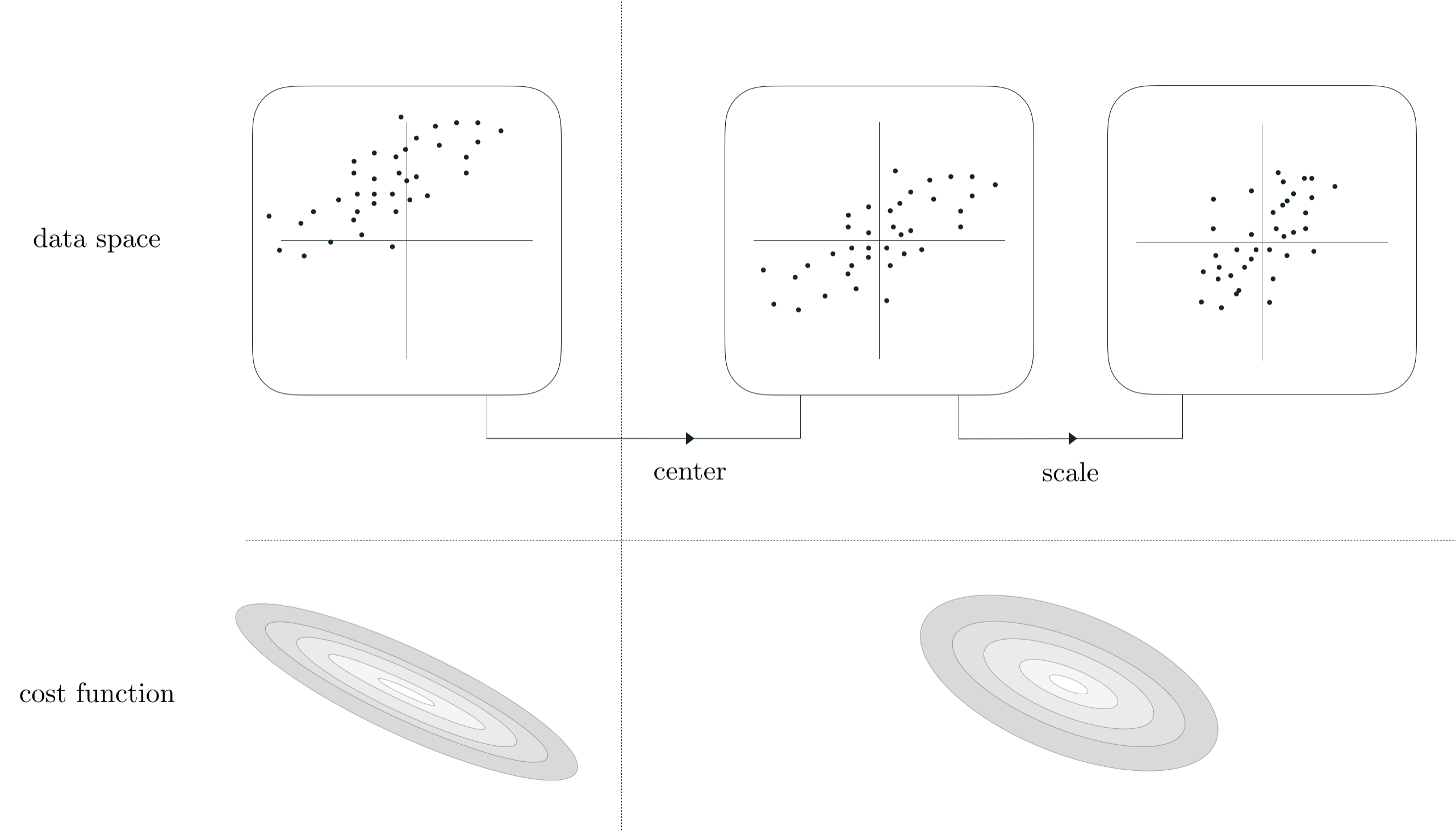
• an extremely simple adjustment of the data ameliorates this issue significantly, called standard normalization

• do the following to each input dimension / feature: subtract mean and divide off standard deviation

• for single input case, we replace each input $x_p$ point with its mean centered unit deviation analog as

\begin{equation} x_p \longleftarrow \frac{x_p - \mu}{\sigma} \end{equation}

where

\begin{equation} \mu = \frac{1}{P}\sum_{p=1}^{P}x_p \\ \end{equation}

and the sample standard deviation of the inputs $\sigma$ is defined as

\begin{array} \ \sigma = \sqrt{\frac{1}{P}\sum_{p=1}^{P}\left(x_p - \mu \right)^2}. \end{array}

• super simple, invertible, and has a profound impact on the shape of our cost function

• lets see what this does to the contours of the cost function we just saw

# show run in both three-dimensions and just the input space via the contour plot
static_plotter.two_input_contour_plot(least_squares_2,[],xmin = -12,xmax = 15,ymin = -5,ymax = 25,num_contours = 7,show_original = False)

• how did the cost function change? lets look at an animation where we slide between the original and standard normalized data

• we will flip through versions of the cost function inputing

\begin{equation} \left(1 - \lambda\right)x_p + \lambda \left( \frac{x_p - \mu}{\sigma} \right) \end{equation}

where $\lambda$ ranges from $0$ (i.e., we use the original input) to $\lambda = 1$

# animation showing cost function transformation from standard to normalized input
scaling_tool = feature_scaling_tools.Visualizer(x,x_normalized,y,'least_squares')
scaling_tool.animate_transition(num_frames=50,xmin = -12,xmax = 15,ymin = -10,ymax = 30,num_contours = 7)

• now lets make the same sort of gradient descent run on the normalized input cost

# show run on contour plot
static_plotter.two_input_contour_plot(g,weight_history,xmin = -3,xmax = 10,ymin = -2,ymax = 6,num_contours = 7,show_original = False)

• much much better!

• how about the resulting fit?

# the original data and best fit line learned from our gradient descent run
ind = np.argmin(cost_history)
least_weights = weight_history[ind]
demo.plot_fit(plotting_weights = [least_weights],colors = ['r'],transformer = normalizer)

• not here - to produce the fit we plug in new test points

• new test points need to be treated precisely as the training data - subtract the same mean / divide by the same std

\begin{equation} \text{normalized_predictor}\left(x\right) = w_0^{\star} + w_1^{\star}\left(\frac{x - \mu}{\sigma}\right). \end{equation}

Example 1. Normalizing the input of a student debt dataset

• does standard normalization work for real data?

• absolutely - e.g., United States student debt dataset

# load data
csvname = datapath + 'student_debt.csv'
data = np.loadtxt(csvname,delimiter = ',')
x = data[:,:-1].T
y = data[:,-1:] 

# plot dataset
demo = regress_plotter.Visualizer(data)
demo.plot_data()

• Least Squares cost before performing standard normalization to input, with run of 25 gradient descent steps

# an implementation of the least squares cost function for linear regression, precisely
# what was shown in Section 8.1 but here pulled in from a backend file
least_squares = cost_lib.choose_cost(x,y,'least_squares')

# run gradient descent to minimize the Least Squares cost for linear regression
g = least_squares; w = np.array([0.0,0.0])[:,np.newaxis]; max_its = 25; alpha_choice = 10**(-7);
weight_history,cost_history = optimizers.gradient_descent(g,alpha_choice,max_its,w)

# show run on contour plot
static_plotter.two_input_contour_plot(g,weight_history,xmin = -0.25,xmax = 0.25,ymin = -0.25,ymax = 0.25,num_contours = 7,show_original = False)

• hugely elliptical! basically impossible to minimize via gradient descent

• because the original input is enormous! so even slight variations from the very best slope/vertical intercept produce huge errors

• corresponding fit will be terrible

# the original data and best fit line learned from our gradient descent run
ind = np.argmin(cost_history)
least_weights = weight_history[ind]
demo.plot_fit(plotting_weights = [least_weights],colors = ['r'])

• after standard normalization, with only $25$ gradient descent steps - with much larger steplength!

# return normalization and inverse normalization functions based on input x
normalizer = standard_normalizer(x)

# normalize input by subtracting off mean and dividing by standard deviation
x_normalized = normalizer(x)

# an implementation of the least squares cost function for linear regression, precisely
# what was shown in Section 8.1 but here pulled in from a backend file
least_squares_2 = cost_lib.choose_cost(x_normalized,y,'least_squares')

# run gradient descent to minimize the Least Squares cost for linear regression
g = least_squares_2; w = np.array([0.0,0.0])[:,np.newaxis]; max_its = 25; alpha_choice = 10**(-1);
weight_history,cost_history = optimizers.gradient_descent(g,alpha_choice,max_its,w)

# show run on contour plot
static_plotter.two_input_contour_plot(g,weight_history,xmin = -1,xmax = 1,ymin = -1,ymax = 1,num_contours = 7,show_original = False,arrows = False)

• way better fit possible

# the original data and best fit line learned from our gradient descent run
ind = np.argmin(cost_history)
least_weights = weight_history[ind]
demo.plot_fit(plotting_weights = [least_weights],colors = ['r'],transformer = normalizer)

8.4.2 Feature scaling for multi-input datasets

• the same standard normalization scheme aids in tuning models for multi-innput regression data as well

• simply do the same thing - mean center and scale by standard deviation - for each input

• normalize the $n^{th}$ input dimension of an $N$-input dimensional dataset $\left\{\mathbf{x}_p,y_p\right\}_{p=1}^N$ as

\begin{equation} x_{p,n} \longleftarrow \frac{x_{p,n} - \mu_n}{\sigma_n} \end{equation}

where

\begin{array} \ \mu_n = \frac{1}{P}\sum_{p=1}^{P}x_{p,n} \\ \sigma_n = \sqrt{\frac{1}{P}\sum_{p=1}^{P}\left(x_{p,n} - \mu_n \right)^2} \end{array}

• see Section notes for examples!

8.4.3 Summary and discussion

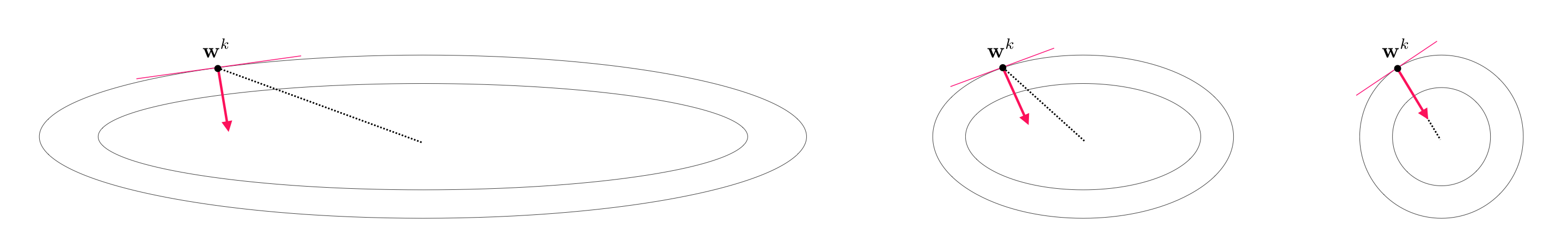
• making the contours of a cost function more 'circular' make it easier to minimize - why?

• e.g., for gradient descent due to the nature of the gradient descent direction!

• this direction points orthogonal to contours - in long narrow valleys this points away from cost minimum, on circular cost it points more towards minimum