Edge histogram based features

Press the button 'Toggle code' below to toggle code on and off for entire this presentation.

from IPython.display import display
from IPython.display import HTML
import IPython.core.display as di # Example: di.display_html('<h3>%s:</h3>' % str, raw=True)

# This line will hide code by default when the notebook is eåxported as HTML
di.display_html('<script>jQuery(function() {if (jQuery("body.notebook_app").length == 0) { jQuery(".input_area").toggle(); jQuery(".prompt").toggle();}});</script>', raw=True)

# This line will add a button to toggle visibility of code blocks, for use with the HTML export version
di.display_html('''<button onclick="jQuery('.input_area').toggle(); jQuery('.prompt').toggle();">Toggle code</button>''', raw=True)

Toggle code

Figure 1: (left panel) A natural image (in this instance of the two creators/writers of the television show 'South Park' (this image is reproduced with permission of Jason Marck). (right panel) The edge-detected version of this image, where the bright yellow pixels indicate large edge content, still describes the scene very well (in the sense that we can still tell there are two people in the image) using only a fraction of the information contained in the original image. Note that edges have been colored yellow for visualization purposes only.

Figure 2: Visual information is processed in an area of the brain where each neuron detects in the observed scene edges of a specific orientation and width. It is thought that what we (and other mammals) "see" is a processed interpolation of these edge detected images.

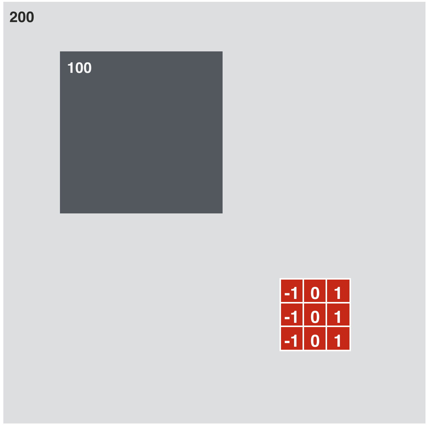
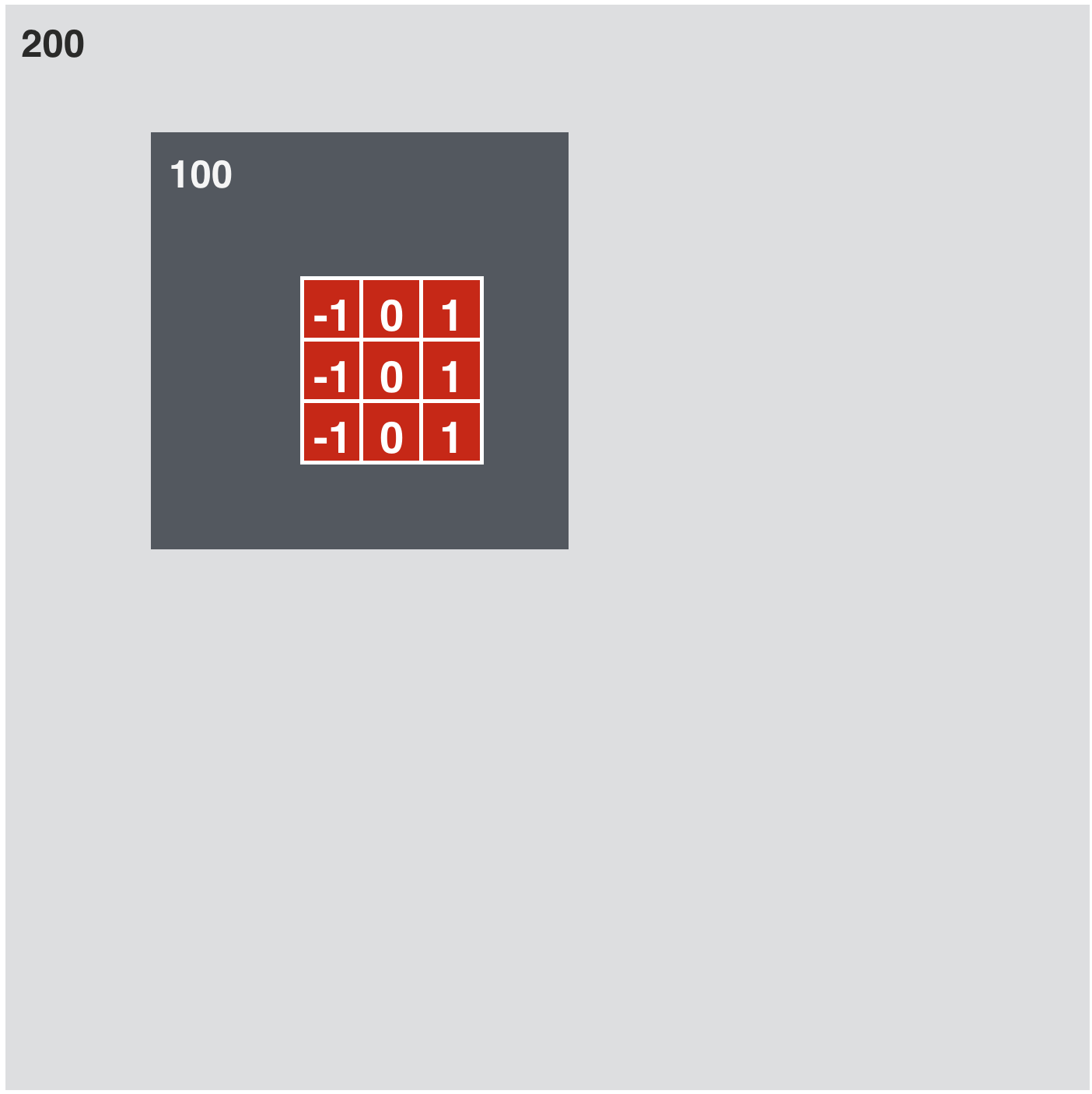
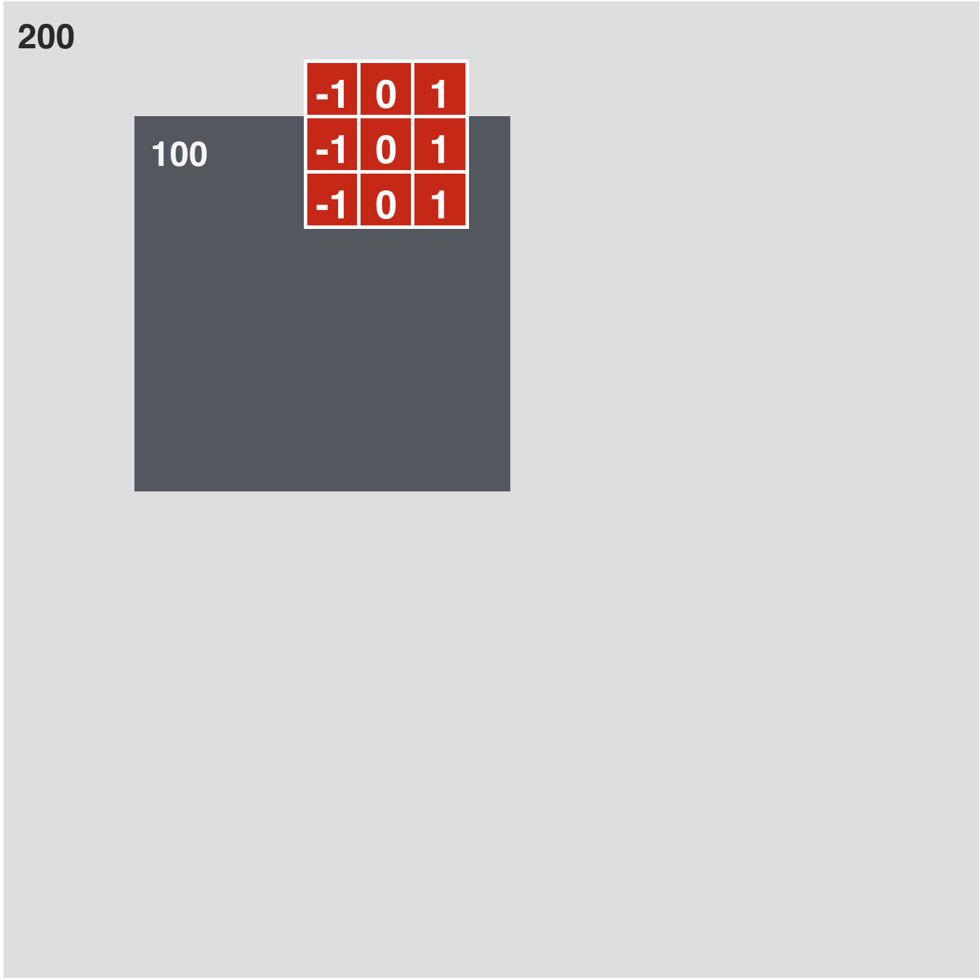
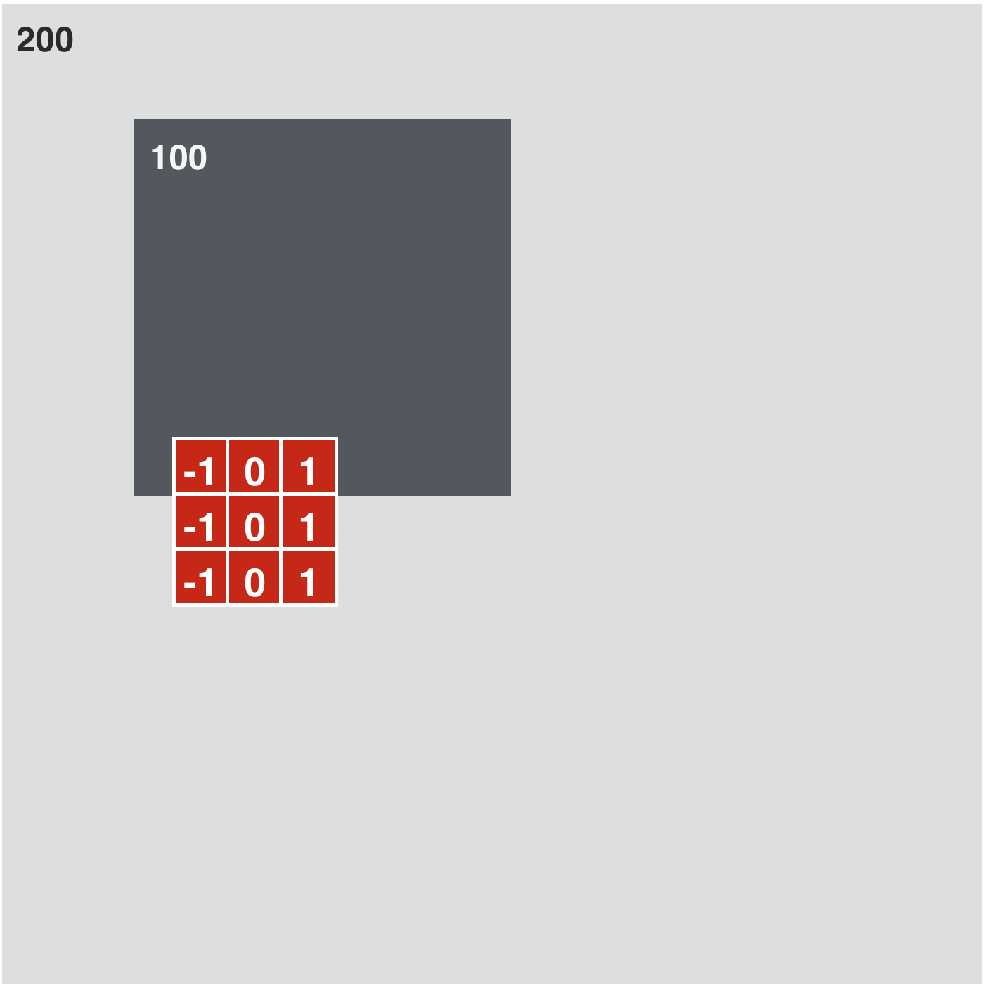
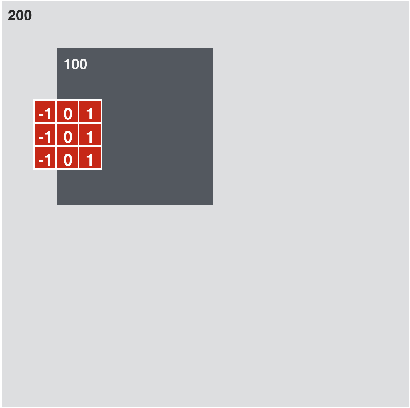
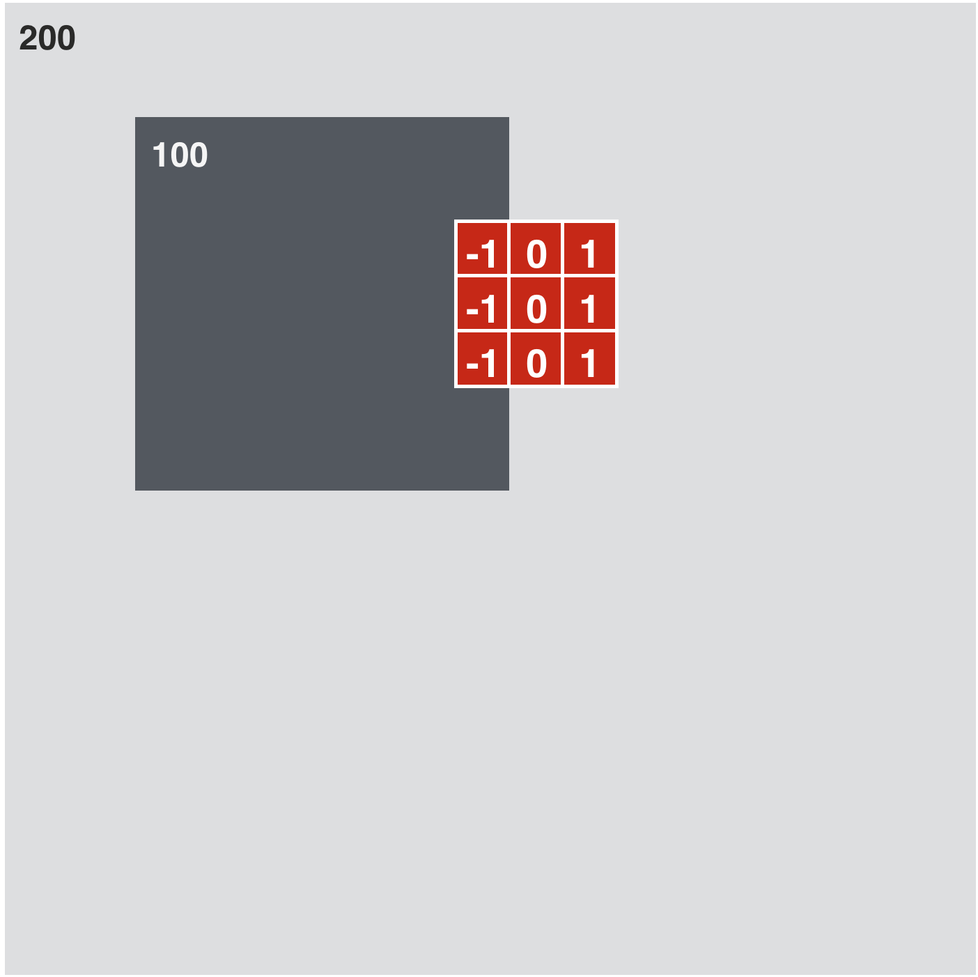
Edge detection via convolution

# load image
image = convlib.image_viz.create_image('square_top')

#w_h = np.array([[-0.5,  0,  0.5]])
#w_v = np.array([[-0.5],
#                [   0],
#                [ 0.5]])

w_h = np.array([[-1, 0, 1],
                [-1, 0, 1],
                [-1, 0, 1]])



kernels = [w_h] 

# compute and plot convolution images
convlib.kernel_viz.show_conv(-image, kernels, contrast_normalization=False)

# load image
image = convlib.image_viz.create_image('square_top')

#w_h = np.array([[-0.5,  0,  0.5]])
#w_v = np.array([[-0.5],
#                [   0],
#                [ 0.5]])


w_v = np.array([[-1, -1, -1],
                [ 0,  0,  0],
                [ 1,  1,  1]])



kernels = [w_v] 

# compute and plot convolution images
convlib.kernel_viz.show_conv(-image, kernels, contrast_normalization=False)

convlib.image_viz.show_conv_kernels()

To capture the total 'edge content' of an image in each direction, we

• I. convolve it with the appropriate kernel

• II. pass the results through a rectified linear unit (ReLU) to remove negative entries

• III. sum up (the remaining positive) pixel values

\begin{equation} f_{i}=\underset{\text{all pixels}}{\sum}\text{max}\left(0,\,w_{i}*x\right) \qquad i=1,\,\ldots,\,8 \end{equation}

Why pass the convolution through ReLU?

# load image
image = convlib.image_viz.create_image('square_top')

w_h = np.array([[-1, 0, 1],
                [-1, 0, 1],
                [-1, 0, 1]])

w_v = np.array([[1, 0, -1],
                [1, 0, -1],
                [1, 0, -1]])



kernels = [w_h, w_v] 

# compute and plot convolution images
convlib.kernel_viz.show_conv(-image, kernels, contrast_normalization=False)

# load image
image = convlib.image_viz.create_image('square_top')


# compute and plot convolution images
convlib.image_viz.show_conv_images(image)

# load image
image = convlib.image_viz.create_image('triangle_top')


# compute and plot convolution images
convlib.image_viz.show_conv_images(image)

# load image
image = cv2.imread('../../mlrefined_images/convnet_images/circle.png',0)
#image = Image.open('../../mlrefined_images/convnet_images/circle.png').convert('L')


# compute and plot convolution images
convlib.image_viz.show_conv_images(image)

# load image
#image = cv2.imread('../../mlrefined_images/convnet_images/star.png', 0)

# downsample the image (if too large)
#image = cv2.resize(image, (0,0), fx=0.25, fy=0.25)

image = Image.open('../../mlrefined_images/convnet_images/star.png').convert('L')
image = image.resize((100,100), Image.ANTIALIAS)

# compute and plot convolution images
convlib.image_viz.show_conv_images(image)

• Real images used in practice are significantly more complicated than these simplistic geometrical shapes and summarizing them using just eight features would be extremely ineffective.

• To fix this issue, instead of computing the edge histogram features over the entire image, we break the image into relatively small patches, and compute features for each patch

\begin{equation} f_{i,\,j}=\underset{j\,\text{th patch}}{\sum}\text{max}\left(0,\,w_{i}*x\right) \qquad i=1,\,\ldots,\,8 \end{equation}

• This is called pooling.

Putting all pieces together: the complete feature extraction pipeline