In this post we describe a very particular form of nonlinear regression called logistic regression that is designed to deal with a very particular kind of dataset that is commonly dealt with in machine learning/deep learning: two-class classification data.
Press the button 'Toggle code' below to toggle code on and off for entire this presentation.
from IPython.display import display
from IPython.display import HTML
import IPython.core.display as di # Example: di.display_html('<h3>%s:</h3>' % str, raw=True)

# This line will hide code by default when the notebook is exported as HTML
di.display_html('<script>jQuery(function() {if (jQuery("body.notebook_app").length == 0) { jQuery(".input_area").toggle(); jQuery(".prompt").toggle();}});</script>', raw=True)

# This line will add a button to toggle visibility of code blocks, for use with the HTML export version
di.display_html('''<button onclick="jQuery('.input_area').toggle(); jQuery('.prompt').toggle();">Toggle code</button>''', raw=True)
1. Logistic regression
In this Section we set the scene for logistic regression by describing the problem setup and how linear regression - as well as reasonable extensions of it - naturally fail with such data.
1.1 The data
- Two class classification is a particular instance of regression or surface-fitting, wherein the output of a dataset of $P$ points $\left\{ \left(\mathbf{x}_{p},y_{p}\right)\right\} _{p=1}^{P}$ is no longer continuous but takes on two fixed numbers.
- We will typically use $y_{p}\in\left\{ -1,\,+1\right\}$.
- How can we perform regression on a dataset like this?
1.2 Trying to fit a discontinuous step function
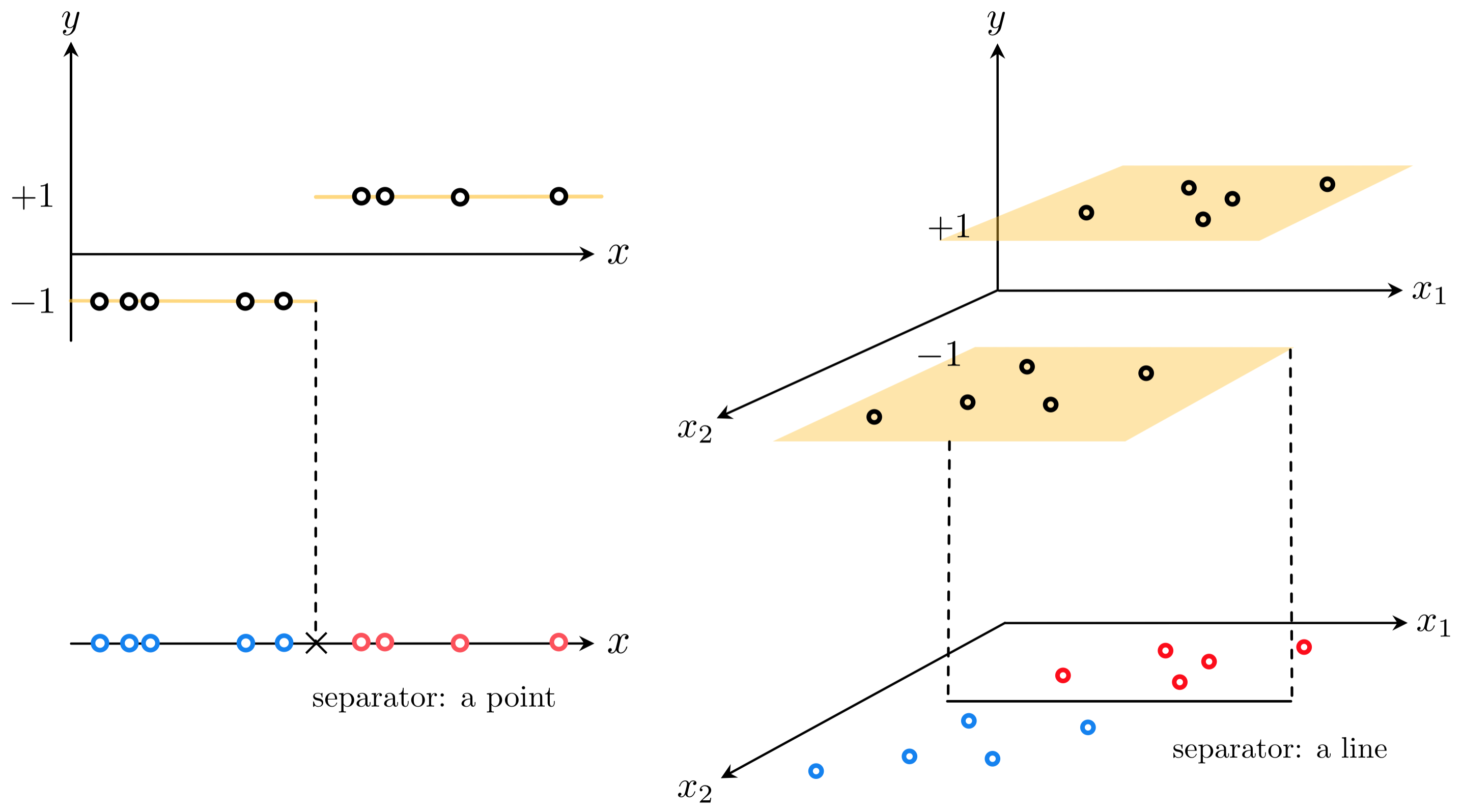
- Lets look at a simple instance when $N = 1$.
- Intuitively fitting a line of the form $y = w_0 + w_1x_{\,}$ to such a dataset will result in an extremely subpar results.
- Ideally we would like to fit a discontinuous step function with a linear boundary to such a dataset. When $N = 1$ it is simply a line $y = w_0 + x_{\,}w_1$ composed with the $\text{sign}(\cdot)$ function
- Remember that the $\text{sign}(\cdot)$ function is defined as $\text{sign}(\alpha) = \begin{cases} +1 \,\,\,\,\,\text{if} \,\, \alpha > 0 \\ -1 \,\,\,\,\,\text{if} \,\, \alpha < 0 \\ \end{cases}$
- How do we tune the parameters of the line?
- We could try to take the lazy way out: first fit the line to the classification dataset via linear regression, then compose the line with the sign function to get a step function fit.
Example 1: Fitting a line first and taking the sign afterward fails to represent a two-class dataset well
# load in dataset
data = np.loadtxt('../../../mlrefined_datasets/superlearn_datasets/2d_classification_data_v1.csv')

# create instance of linear regression demo, used below and in the next examples
demo1 = superlearn.logistic_regression_simple_demos.visualizer(data)
demo1.run_algo(algo = 'newtons_method',w_init = [-1,-1], max_its = 1)

# plot dataset
demo1.naive_fitting_demo()

- We need to tune the parameters of $\text{sign}\left(w_0 + x_{\,}w_1 \right)$.
- How? we can try to setup a proper Least Squares function.
- Take a single point $\left(x_p,\,y_p \right)$. We would ideally like for its evaluation to match its label value
- And of course we would like this to hold for every point
Example 2: Visualizing the counting cost on a simple dataset
# create an instance of the visualizer and plot
demo2 = superlearn.cost_viewer.Visualizer(data)
demo2.plot_costs(viewmax = 25,view = [20,125])

1.2 Introducing the hyperbolic tangent function and a logistic Least Squares
- We cannot directly fit a discontinuous step function to our data.
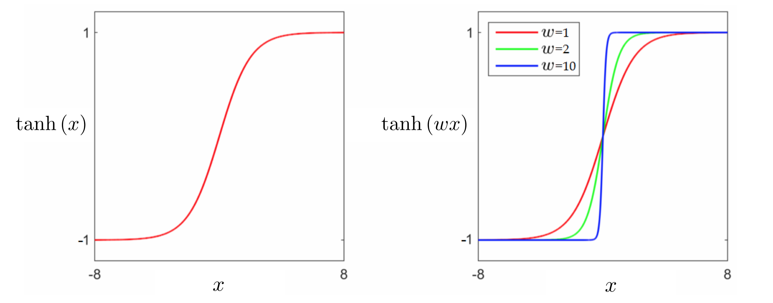
Swapping out the sign function with tanh
\begin{equation} \text{tanh}\left(w_0 + x_pw_1 \right) = y_p \end{equation}Using the same logic we can form the following Least Squares cost for logistic regression
\begin{equation} g(w_0,w_1) = \sum_{p=1}^P \left(\text{tanh}\left(w_0 + x_pw_1 \right) - y_p \right)^2 \end{equation}This cost function can indeed be minimized using local methods, but it is non-convex and contains large flat regions which limits our choice of algorithms to normalized gradient descent.
1.3 The convex logistic regression
Recall our desired equality for the $p^{th}$ point
\begin{equation} \text{tanh}\left(w_0 + x_pw_1 \right) = y_p \end{equation}Because tanh is an odd function - that is $\text{tanh}\left(s\right) = -\text{tanh}\left(-s\right)$ for all $s$ - and because $y_{p}\in\left\{ -1,\,+1\right\}$, we can write this as
\begin{equation} \text{tanh}\left(y_p\left(w_0 + xw_1\right)\right) = 1 \end{equation}Now we can use the exponential definition of tanh, $\text{tanh}\left(s\right) = \frac{2}{1 + e^{-s}}-1$ to rewrite each desired equality equivalently as
\begin{equation} 1 + e^{-y_p\left(w_0 + xw_1\right)} = 1 \end{equation}From there we could either subtract one off of both sides to give equivalently
\begin{equation} e^{-y_p\left(w_0 + xw_1\right)} = 0 \end{equation}or take the log of both sides to give
\begin{equation} \text{log}\left(1 + e^{-y_p\left(w_0 + xw_1\right)}\right) = 0 \end{equation}Both options provide an equivalent way of expressing the desired equality, are nonnegative, and can be used to form convex cost functions for logistic regression.
e.g., the latter expressions gives the commonly used softmax (also called the log-loss) cost function
\begin{equation} g\left(w_0,w_1\right) = \sum_{p=1}^P\text{log}\left(1 + e^{-y_p\left(w_0 + x_pw_1\right)}\right) \end{equation}- The softmax cost function is convex, so we can apply (unnormalized) gradient descent (and other algorithms) more easily
- For all these reasons, the softmax cost is more widely used in practice for logistic regression than the logistic Least Squares cost.
Example 4: Using unnormalized gradient descent to perform logistic regression using the softmax cost
# define the input and output of our dataset
x = data[:,0]
x.shape = (len(x),1)
y = data[:,1]
y.shape = (len(y),1)

# the convex softmax cost function
def softmax(w):
    cost = 0
    for p in range(0,len(y)):
        x_p = x[p,:]
        y_p = y[p]
        cost += np.log(1 + np.exp(-y_p*(w[0] + w[1]*x_p)))
    return cost
# declare an instance of our current our optimizers
opt = superlearn.optimimzers.MyOptimizers()

# run desired algo with initial point, max number of iterations, etc.,
w_hist = opt.gradient_descent(g = softmax,w = np.asarray([3.0,3.0]),version = 'unnormalized',max_its = 25, alpha = 1)

# create instance of logisic regression demo and load in data, cost function, and descent history
demo4 = superlearn.classification_2d_demos.Visualizer(data,softmax)

# animate descent process
demo4.animate_run(w_hist,num_contours = 25,viewmax = 7)
How about when $N>1$?
Using the same logic that led us to the softmax cost when $N = 1$, we can derive the same set of desired equalities more generally with $N>1$ inputs
\begin{equation} \text{log}\left( 1 + e^{-y_p\left(w_{0}+ x_{1,p}w_{1} + x_{2,p}w_{2} + \cdots +x_{N,p}w_{N}\right)} \right) = 0 \end{equation}Using the more compact vector notation
\begin{equation} \mathbf{w}=\left[\begin{array}{c} w_{1}\\ w_{2}\\ \vdots\\ w_{N} \end{array}\right] \,\,\,\,\,\text{and}\,\,\,\,\,\, \mathbf{x}_p=\left[\begin{array}{c} x_{1,p}\\ x_{2,p}\\ \vdots\\ x_{N,p} \end{array}\right] \end{equation}we can write the above more compactly via the inner product as
\begin{equation} \text{log}\left(1 + e^{-y_p^{\,}\left(w_0+\mathbf{x}_p^T \mathbf{w}_{\,}^{\,}\right)}\right) = 0 \end{equation}Softmax for general $N$
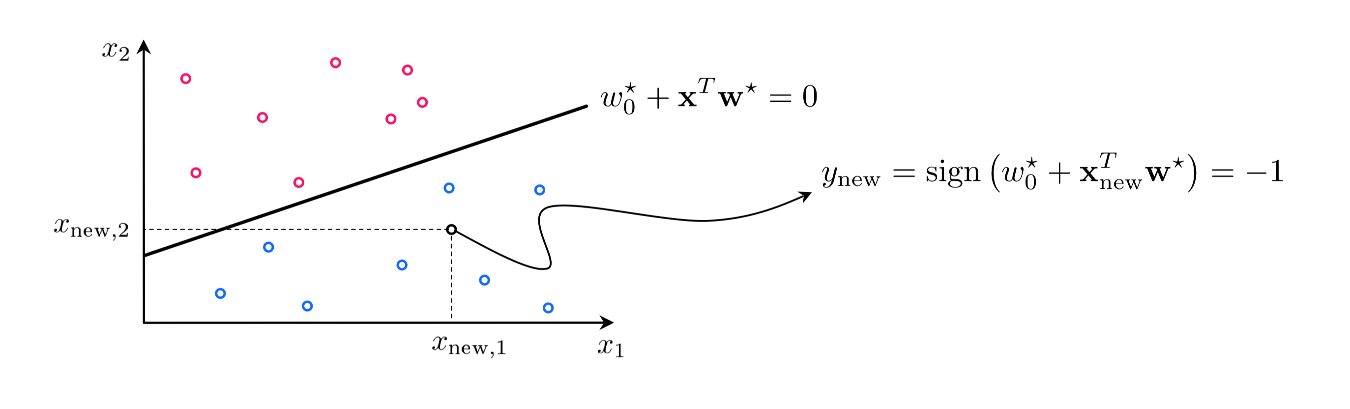
- While logistic regression fits a nonlinear surface to classification data in the input-output space, the decision boundary in the input space is always linear - a hyperplane defined by
- Hence logistic regression is considered a linear classifier.
Example 7: Noisy classification datasets are so typical they are almost the norm
# load in dataset
data = np.loadtxt('../../mlrefined_datasets/superlearn_datasets/3d_classification_data_v0.csv',delimiter = ',')

# create instance of linear regression demo, used below and in the next examples
demo7 = superlearn.classification_3d_demos.Visualizer(data)

# plot data
demo7.plot_data(view = [15,-140])

In the context of classification a 'noisy' point is one that has an incorrect label (noisy datasets are very common in practice).
# define the input and output of our dataset - assuming arbitrary N > 2 here
x = data[:,:-1]
y = data[:,-1]
y.shape = (len(y),1)

# the convex softmax cost function - for N > 2
def softmax(w):
    cost = 0
    for p in range(0,len(y)):
        x_p = x[p,:]
        y_p = y[p]
        a_p = w[0] + sum([a*b for a,b in zip(w[1:],x_p)])
        cost += np.log(1 + np.exp(-y_p*a_p))
    return cost

# declare an instance of our current our optimizers
opt = superlearn.optimimzers.MyOptimizers()

# run desired algo with initial point, max number of iterations, etc.,
w_hist = opt.newtons_method(g = softmax,w = np.random.randn(3,1),max_its = 5)

# create instance of 3d demos
demo8 = superlearn.classification_3d_demos.Visualizer(data)

# draw the final results
demo8.static_fig(w_hist,view = [15,-140])

Another noisy example
# load in dataset
data = np.loadtxt('../../mlrefined_datasets/superlearn_datasets/3d_classification_data_v2.csv',delimiter = ',')

# create instance of linear regression demo, used below and in the next examples
demo9 = superlearn.classification_3d_demos.Visualizer(data)

# plot data
demo9.plot_data(view = [25,-60])

# define the input and output of our dataset - assuming arbitrary N > 1 here
x = data[:,:-1]
y = data[:,-1]
y.shape = (len(y),1)

# declare an instance of our current our optimizers
opt = superlearn.optimimzers.MyOptimizers()

# run desired algo with initial point, max number of iterations, etc.,
w_hist = opt.newtons_method(g = softmax,w = np.random.randn(3,1),max_its = 5)

# create instance of 3d demos
demo10 = superlearn.classification_3d_demos.Visualizer(data)

# draw the final results
demo10.static_fig(w_hist,view = [25,-60])

1.4 Classification nomenclature and predictions
1.5 Counting misclassifications and the accuracy of a trained classifier
Because $y_p \in \{\pm 1\}$
\begin{equation} \left(\text{sign}\left(w_0+\mathbf{x}_p^T\mathbf{w}_{\,}^{\,} \right) - y_p \right)^2 = \begin{cases} 0 \,\,\,\, \text{if} \,\,\,\text{sign}\left(w_0+\mathbf{x}_p^T\mathbf{w}_{\,}^{\,} \right) = y_p \\ 4 \,\,\,\, \text{else} \\ \end{cases} \end{equation}Therefore to count the total number of misclassifications of a trained classifier we can simply evaluate the counting cost, dividing by $4$ as
\begin{equation} \text{number of misclassifications} = \frac{1}{4}\sum_{p=1}^P \left(\text{sign}\left(w_0^{\star}+\mathbf{x}_p^T\mathbf{w}_{\,}^{\star} \right) - y_p \right)^2 \end{equation}Example 9: Comparing the softmax cost and the counting cost
# load in dataset
data = np.loadtxt('../../mlrefined_datasets/superlearn_datasets/3d_classification_data_v2.csv',delimiter = ',')

# create instance of cost comparison demo
demo11 = superlearn.cost_comparisons.Visualizer(data)

# run
demo11.compare_to_counting(cost = 'softmax',max_its = 50,num_runs = 3,alpha = 10**-2,algo = 'gradient_descent')

Note: during optimization one should save the weight associated with the lowest number of misclassifications not the lowest cost value.
The simplest measure of how well a classifier has been trained on a set of $P$ training datapoints is its accuracy
\begin{equation} \text{accuracy}= 1 - \frac{1}{4P}\sum_{p=1}^P \left(\text{sign}\left(w_0^{\star}+\mathbf{x}_p^T\mathbf{w}_{\,}^{\star} \right) - y_p \right)^2 \end{equation}which ranges from 0 (no points classified correctly) to 1 (all points classified correctly).